Week 8
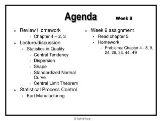
Agenda. Week 8. Review Homework Chapter 4 – 2, 3 Lecture/discussion Statistics in Quality Central Tendency Dispersion Shape Standardized Normal Curve Central Limit Theorem Statistical Process Control Kurt Manufacturing. Week 9 assignment Read chapter 5 Homework

Week 8
E N D
Presentation Transcript
Agenda Week 8 • Review Homework • Chapter 4 – 2, 3 • Lecture/discussion • Statistics in Quality • Central Tendency • Dispersion • Shape • Standardized Normal Curve • Central Limit Theorem • Statistical Process Control • Kurt Manufacturing • Week 9 assignment • Read chapter 5 • Homework • Problems: Chapter 4 - 8, 9, 24, 26, 36, 44, 49 Statistics
The Use of Statistics in Quality Chapter Four Statistics
A few notes on SPC’s historical background • Walter Shewhart (Bell Labs 1920s) - suggested that every process exhibits some degree of variation and therefore is expected. • identified two types of variation (chance cause) and (assignable cause) • proposed first control chart to separate these two types of variation. • SPC was successfully applied during World War II as a means of insuring interchangeability of parts for weapons/ equipment. • Resurgence of SPC in the 1980s in response to Japanese manufacturing success. Statistics
The basics • “Don’t inspect the product, inspect the process.” • “You can’t inspect it in, you’ve got to build it in.” • “If you can’t measure it, you can’t manage it.” Statistics
Barriers to process control • Tendency to focus on volume of output rather than quality of output. • Tendency to measure products against a set of internal conformance specifications that may or may not relate to customer expectations. Statistics
The SPC approach • The SPC approach is designed to identify underlying cause of problems which cause process variations that are outside predetermined tolerances and to implement controls to fix the problem. Statistics
The SPC steps Basic approach: • Awareness that a problem exists. • Determine the specific problem to be solved. • Diagnose the causes of the problem. • Determine and implement remedies. • Implement controls to hold the gains achieved by solving the problem. Statistics
SPC requires the use of statistics • Quality improvement efforts have their foundation in statistics. • Statistical process control involves the • collection • tabulation • analysis • interpretation • presentation of numerical data. Statistics
Statistic types • Deductive statistics describe a complete data set • Inductive statistics deal with a limited amount of data Statistics
Statistics Parameters:2 Inferential Statistics POPULATION Deductive SAMPLE Statistics: x, s, s2 Inductive Statistics
Types of data ` • Variables data - quality characteristics that are measurable values. • Measurable and normally continuous; may take on any value. • Attribute data - quality characteristics that are observed to be either present or absent, conforming or nonconforming. • Countable and normally discrete; integer Statistics
Descriptive statistics • Measures of Central Tendency • Describes the center position of the data • Mean Median Mode • Measures of Dispersion • Describes the spread of the data • Range Variance Standard deviation Statistics
Measures of central tendency: Mean Arithmetic mean x = • where xi is one observation, means “add up what follows” and N is the number of observations So, for example, if the data are : 0,2,5,9,12 the mean is (0+2+5+9+12)/5 = 28/5 = 5.6 Statistics
Measures of central tendency: Median - mode • Median = the observation in the ‘middle’ of sorted data • Mode = the most frequently occurring value Statistics
Median and mode 100 91 85 84 75 72 72 69 65 Mode Median Mean = 79.22 Statistics
Measures of dispersion: range • The range is calculated by taking the maximum value and subtracting the minimum value. 2 4 6 8 10 12 14 Range = 14 - 2 = 12 Statistics
Measures of dispersion: variance • Calculate the deviation from the mean for every observation. • Square each deviation • Add them up and divide by the number of observations Statistics
Measures of dispersion: standard deviation • The standard deviation is the square root of the variance. The variance is in “square units” so the standard deviation is in the same units as x. Statistics
Standard deviation and curve shape • If is small, there is a high probability for getting a value close to the mean. • If is large, there is a correspondingly higher probability for getting values further away from the mean. Statistics
Chebyshev’s theorem • If a probability distribution has the mean and the standard deviation , the probability of obtaining a value which deviates from the mean by at least k standard deviations is at most 1/k2. Statistics
As a result Probability of obtaining a value beyond “x” standard deviations is at most:: 2 standard deviations 1/22 = 1/4 = 0.25 3 standard deviations 1/32 = 1/9 = 0.11 4 standard deviations • 1/42 = 1/16 = 0.0625 Statistics
Other measures of dispersion: skewness • When a distribution lacks symmetry, it is considered skewed. • <0 left 0 = symmetrical >0 right Statistics
Other measures of dispersion: kurtosis • suggests “peakedness” of the data • “a” can be used to compare distributions Statistics
The normal frequency distribution Statistics
The normal curve • A normal curve is symmetrical about • The mean, mode, and median are equal • The curve is uni-modal and bell-shaped • Data values concentrate around the mean • Area under the normal curve equals 1 Statistics
The normal curve • If x follows a bell-shaped (normal) distribution, then the probability that x is within • 1 standard deviation of the mean is 68% • 2 standard deviations of the mean is 95 % • 3 standard deviations of the mean is 99.7% Statistics
One standard deviation 68.3% Statistics
Two standard deviations 2 2 95.5% Statistics
Three standard deviations 3 3 99.73% Statistics
The standardized normal = 0 = 1 x scale -3 -2 - + +2 +3 z scale -3 -2 -1 0 +1 +2 +3 Statistics

