Download
1 / 14
190 likes | 946 Vues
Cumene Oxidation and Hydrolysis. 4. 1. 2. 3. Cumene Oxidation - Chain Reaction Sequence. 10 -3 s -1. Cumene Oxidation – Rate Equations. The following equations describe the rate of production / consumption of the key process variables in terms of measurable experimental quantities.

E N D
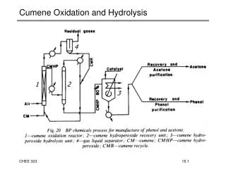
Cumene Oxidation and Hydrolysis 4 1 2 3
Cumene Oxidation – Rate Equations • The following equations describe the rate of production / consumption of the key process variables in terms of measurable experimental quantities.
Batch Process Dynamics Under Kinetic Control • Commodities are not produced batch-wise, but insight can be gained by examining batch reaction dynamics. • The simplest simulation ignores mass transfer by setting [O2] to its equilibrium value, and integrating the system of ODE’s numerically to predict how the reagent and product concentrations will evolve as a function of time.
Batch Process Dynamics Under Kinetic Control • These coupled ODE’s are solved by numerical integration, as illustrated below:
Batch Process Dynamics Under Kinetic Control • Assuming that oxygen can be maintained at its equilibrium concentration, here is the evolution of a batch process with [Fe2+]o=0.1M, [ROOH]o=0.001M in a cumene solution ([RH]o=6.7M) • Since the process is quite exothermic, this reaction rate is far too high for large-scale contactors.
Batch Process Dynamics Under Kinetic Control • It is interesting to note the insensitivity of batch dynamics to the initial hydroperoxide concentration. Consider these two reactions, each simulated with [Fe2+]o=0.1M, [RH]o=6.7M: • [ROOH]o=0.001M [ROOH]o=0.1M
Semi-batch Dynamics Under Kinetic Control • More manageable reaction velocities can be achieved by metering the initiator such that its overall concentration is constant. This simulation used [ROOH]o=0.001M, [RH]o=6.7M with [Fe2+]=0.0017M, and [O2]=0.009 M maintained throughout. • This process would require about 18 batches of 11m3 each day to produce 50,000 tonnes pa.
PFR Dynamics Under Kinetic Control • Process economics will be improved by • operating with continuous plug flow • reactor configuration. The relevant • design equations, expressed in • terms of space time, are as follows: • These assume perfect plug flow, isothermal operation and ideal oxygen transport across the gas-liquid interface.
PFR Dynamics Under Kinetic Control • This simulation models four PFR’s in series, each injecting [Fe2+]=0.005M at the column’s entrance. Mass transfer effects are ignored for the time being. • This simple arrangement of four identical PFR’s gives an overall conversion of 0.44, and requires each reactor to be 1.2 m3 total volume (assuming liquid hold-up=0.75) to give 50,000 tonnes pa.
CSTR Dynamics Under Kinetic Control • The CSTR design problem is significantly • different from the batch/PFR cases, but • is relatively simple if mass transfer is • assumed to be ideal. • The first two equations can be solved, given inlet concentrations and a space time, to predict the product stream composition. The functions for d[RH]/dt and d[Fe2+]/dt are those expressed in slide 16.3.
CSTR Dynamics Under Kinetic Control • It is interesting to note that the CSTR actually outperforms the PFR configuration for this auto-initiating oxidation • Since [ROOH] remains at a high steady-state value, the CSTR does not suffer from an induction period, and initiator is supplied continuously to keep the process going. • In these examples, Fe2+ is • added at a total concentration • of 0.1M. Note how the • process performances • converge at longer space • times. • Using a space time of 10 min • to achieve a conversion of 0.57, • a single 1m3 CSTR could • produce 50,000 tonnes pa.
PFR Dynamics – Exceptional Mass Transport Ideal mass transfer; klA/V= Conversion = 0.15 Great mass transfer; klA/V=3.5 s-1 Conversion = 0.08
PFR Dynamics – Conventional Mass Transport Ideal mass transfer; klA/V= Conversion = 0.15 Good mass transfer; klA/V=0.35 s-1 Conversion = 0.01