Understanding Linear Models with Categorical Predictors: Analyzing Gender Differences in RT
620 likes | 757 Vues
This analysis delves into the application of linear models involving categorical predictors, particularly focusing on gender differences and reaction times (RT). Using simulated data, we explore how categorical variables impact response outcomes. The output from linear regression models illustrates significant differences between groups, highlighting statistical relevance. By transforming and releveling categorical predictors, we can gain insights into how different reference levels affect the understanding of data. This comprehensive approach serves as a guide to analyzing categorical variables within linear modeling.

Understanding Linear Models with Categorical Predictors: Analyzing Gender Differences in RT
E N D
Presentation Transcript
More on the linearmodel Categorical predictors
men RT ~ Noise + Gender women
Demo set.seed(666) pred = c(rep(0,20),rep(1,20)) resp = c(rnorm(20,mean=2,sd=1), rnorm(20,mean=2,sd=1)) for(i in 1:10){ resp = c(resp[1:20],resp[21:40]+1) plot(resp~pred, xlim=c(-1,2),ylim=c(0,14),xaxt="n",xlab="") axis(side=1,at=c(0,1),labels=c("A","B")) text(paste("mean B\nequals:",i,sep="\n"), x=-0.5,y=10,cex=1.5,font=2) abline(lm(resp~pred)) Sys.sleep(1.25) }
Deep idea: A categorical difference between two groups can be expressed as a line going fromone group to another
Continuous predictor … units up 1 unit “to the right”
Continuous predictor … units up 1 unit “to the right”
Categorical predictor … units up F M 1 category “to the right”
Output: categorical predictor > summary(lm(RT ~ gender)) Call: lm(formula = RT ~ gender) Residuals: Min 1Q Median 3Q Max -231.039 -39.649 2.999 44.806 155.646 Coefficients: Estimate Std. Error t value Pr(>|t|) (Intercept) 349.203 4.334 80.57 <2e-16 *** genderM 205.885 6.129 33.59 <2e-16 *** --- Signif. codes: 0 ‘***’ 0.001 ‘**’ 0.01 ‘*’ 0.05 ‘.’ 0.1 ‘ ’ 1 Residual standard error: 61.29 on 398 degrees of freedom Multiple R-squared: 0.7392, Adjusted R-squared: 0.7386 F-statistic: 1128 on 1 and 398 DF, p-value: < 2.2e-16
Output: categorical predictor > summary(lm(RT ~ gender)) Call: lm(formula = RT ~ gender) Residuals: Min 1Q Median 3Q Max -231.039 -39.649 2.999 44.806 155.646 Coefficients: Estimate Std. Error t value Pr(>|t|) (Intercept) 349.203 4.334 80.57 <2e-16 *** genderM 205.885 6.129 33.59 <2e-16 *** --- Signif. codes: 0 ‘***’ 0.001 ‘**’ 0.01 ‘*’ 0.05 ‘.’ 0.1 ‘ ’ 1 Residual standard error: 61.29 on 398 degrees of freedom Multiple R-squared: 0.7392, Adjusted R-squared: 0.7386 F-statistic: 1128 on 1 and 398 DF, p-value: < 2.2e-16
REFERENCE LEVEL
But what happens… … when I have more than two groups or categories?
Output: three groups Females = 349.203 (intercept) Males = 349.203 + 205.885 Infants = 349.203 + 203.983 > summary(lm(RT ~ gender)) Call: lm(formula = RT ~ gender) Residuals: Min 1Q Median 3Q Max -231.039 -41.055 3.404 38.428 155.646 Coefficients: EstimateStd. Error t value Pr(>|t|) (Intercept) 349.203 4.228 82.59 <2e-16 *** genderM 205.885 5.979 34.43 <2e-16 *** genderI 203.983 5.979 34.11 <2e-16 *** --- Signif. codes: 0 ‘***’ 0.001 ‘**’ 0.01 ‘*’ 0.05 ‘.’ 0.1 ‘ ’ 1 Residualstandarderror: 59.79 on 597 degrees of freedom MultipleR-squared: 0.724, AdjustedR-squared: 0.7231 F-statistic: 783.1 on 2 and 597 DF, p-value: < 2.2e-16
REFERENCE LEVEL
Output: changing reference level Infants = 553.185 (intercept) Females = 553.185 – 203.983 Males = 553.185 + 1.903 > summary(lm(RT ~ gender)) Call: lm(formula = RT ~ gender) Residuals: Min 1Q Median 3Q Max -231.039 -41.055 3.404 38.428 155.646 Coefficients: EstimateStd. Error t value Pr(>|t|) (Intercept) 553.185 4.228 130.835 <2e-16 *** genderF -203.983 5.979 -34.114 <2e-16 *** genderM 1.903 5.979 0.318 0.75 --- Signif. codes: 0 ‘***’ 0.001 ‘**’ 0.01 ‘*’ 0.05 ‘.’ 0.1 ‘ ’ 1 Residualstandarderror: 59.79 on 597 degrees of freedom MultipleR-squared: 0.724, AdjustedR-squared: 0.7231 F-statistic: 783.1 on 2 and 597 DF, p-value: < 2.2e-16 Notice that nothing has really changed… it’s just a different perspective on the same data
REFERENCE LEVEL
In case you need it:Releveling: In R relevel(myvector, ref="mynew_reference_level”)
More on the linearmodel Centering and standardization
Output: weird intercept > summary(lm(familiarity ~ word_frequency)) Call: lm(formula = familiarity ~ word_frequency) Residuals: Min 1Q Median 3Q Max -4.5298 -1.2306 -0.0087 1.1141 4.6988 Coefficients: Estimate Std. Error t value Pr(>|t|) (Intercept) -2.790e+00 6.232e-01 -4.477 9.37e-06 *** word_frequency 1.487e-04 1.101e-05 13.513 < 2e-16 *** --- Signif. codes: 0 ‘***’ 0.001 ‘**’ 0.01 ‘*’ 0.05 ‘.’ 0.1 ‘ ’ 1 Residual standard error: 1.699 on 498 degrees of freedom Multiple R-squared: 0.2683, Adjusted R-squared: 0.2668 F-statistic: 182.6 on 1 and 498 DF, p-value: < 2.2e-16
Uncentered > summary(lm(familiarity ~ word_frequency)) Call: lm(formula = familiarity ~ word_frequency) Residuals: Min 1Q Median 3Q Max -4.5298 -1.2306 -0.0087 1.1141 4.6988 Coefficients: Estimate Std. Error t value Pr(>|t|) (Intercept) -2.790e+00 6.232e-01 -4.477 9.37e-06 *** word_frequency1.487e-04 1.101e-05 13.51 <2e-16 *** --- Signif. codes: 0 ‘***’ 0.001 ‘**’ 0.01 ‘*’ 0.05 ‘.’ 0.1 ‘ ’ 1 Residual standard error: 1.699 on 498 degrees of freedom Multiple R-squared: 0.2683, Adjusted R-squared: 0.2668 F-statistic: 182.6 on 1 and 498 DF, p-value: < 2.2e-16
Centered > summary(lm(familiarity ~ word_frequency.c)) Call: lm(formula = familiarity ~ word_frequency.c) Residuals: Min 1Q Median 3Q Max -4.5298 -1.2306 -0.0087 1.1141 4.6988 Coefficients: Estimate Std. Error t value Pr(>|t|) (Intercept) 5.568e+00 7.598e-02 73.28 <2e-16 *** word_frequency.c1.487e-04 1.101e-05 13.51 <2e-16 *** --- Signif. codes: 0 ‘***’ 0.001 ‘**’ 0.01 ‘*’ 0.05 ‘.’ 0.1 ‘ ’ 1 Residual standard error: 1.699 on 498 degrees of freedom Multiple R-squared: 0.2683, Adjusted R-squared: 0.2668 F-statistic: 182.6 on 1 and 498 DF, p-value: < 2.2e-16
Centered and scaled is now in standard deviations
Centering vs. Standardization • Centering = subtracting the mean of the data from the data mydata = mydata - mean(mydata) • Standardization = subtracting the mean of the data from the data and then dividing by the standard deviation mydata = (mydata- mean(mydata))/ sd(mydata)
Centering vs. Standardization • Centering = subtracting the mean of the data from the data mydata = mydata - mean(mydata) • Standardization = subtracting the mean of the data from the data and then dividing by the standard deviation mydata = scale(mydata)
Centering vs. Standardization • Centering = often leads to more interpretable coefficients; doesn’t change metric mydata = mydata - mean(mydata) • Standardization = gets rid of the metric (is then in standard units) and then dividing by the standard deviation mydata = (mydata- mean(mydata))/ sd(mydata) Standardization is also often called z-scoring and sometimes normalization (but you should not call it that way)
“Standardization” is a linear transformation … which means it doesn’t really do anything to your results
Linear Transformations • Seconds Milliseconds • Word Frequency Word Frequency by 1000 • Centering, Standardization None of these change the “significance”, only the metric of the coefficients
More on the linearmodel Interactions
"Usually (but not always) the interaction, if it is present, will be the most interesting thing going on." Jack Vevea, UC Merced
Main Effects InteractionEffects
One main effect smallpictures RT (ms) largepictures NearSentFarSent
Two main effects smallpictures largepictures RT (ms) NearSentFarSent
Interaction #1 smallpictures RT (ms) largepictures NearSentFarSent
Interaction #2 smallpictures largepictures RT (ms) NearSentFarSent
Interaction #3 smallpictures largepictures RT (ms) NearSentFarSent
Interaction #4 smallpictures largepictures RT (ms) NearSentFarSent