Download
1 / 27
270 likes | 474 Vues
On Wind-Driven Electrojets at Magnetic Cusps in the Nightside Ionosphere of Mars M. O. Fillingim 1 , R. J. Lillis 1 , S. L. England 1 , L. M. Peticolas 1 , D. A. Brain 1 , J. S. Halekas 1 , C. Paty 2 , D. Lummerzheim 3 , and S. W. Bougher 4

E N D
On Wind-Driven Electrojets at Magnetic Cusps in the Nightside Ionosphere of Mars M. O. Fillingim1, R. J. Lillis1, S. L. England1, L. M. Peticolas1, D. A. Brain1, J. S. Halekas1, C. Paty2, D. Lummerzheim3, and S. W. Bougher4 1Space Sciences Laboratory, University of California, Berkeley 2School of Earth and Atmospheric Sciences, Georgia Institute of Technology, Atlanta 3Geophysical Institute, University of Alaska, Fairbanks 4Department of Atmospheric, Oceanic and Space Sciences, University of Michigan, Ann Arbor 5th Alfven Conference Sapporo, Japan 5 October 2010
Outline Summary Martian Magnetic Fields and Cusps Martian Ionospheric Dynamo Martian Ionospheric Currents Terrestrial Auroral Electrojets Martian Auroral Electrojets Variability Caveats/Assumptions/Simplifications Summary
Summary • The complex magnetic topology at Mars allows solar wind (and accelerated) electrons to ionize the nightside atmosphere in limited regions (cusps) forming a patchy nightside ionosphere • Neutral winds drive ionospheric currents at altitudes where ions are collisionally coupled to the neutral atmosphere while electrons are magnetized dynamo region • Inhomogeneities in the ionospheric conductivity lead to polarization electric fields and secondary ionospheric currents – secondary currents can reinforce original currents forming electrojets • The magnetic signatures of electrojets can be measured from orbit and from the surface
Martian Magnetic Fields and Cusps • No global magnetic field but strong crustal fields • Cusps form where radial crustal fields connect to the IMF • solar wind has access to the atmosphere ionization • Non-uniform global distribution of cusps and ionization • Accelerated electrons, ionospheric structure, and aurora associated with cusps Probability of observing loss cones on the nightside Radial component of B
Martian Ionospheric Dynamo • Ionospheric currents exist where ions are collisional (i < in) but electrons are magnetized (e > en) dynamo region • Crustal magnetic fields alter the ionospheric electrodynamics • The altitude of the dynamo is geographically dependent • Currents vary on the same spatial scales as the crustal fields do at ionospheric altitudes (~ 100 – 600 km)
Martian Ionospheric Currents • (see Fillingimet al. (2010), Icarus, 206(1), pp. 112-119.) • 1. Start with observed electron energy spectra Electron spectrogram observed by Mars Global Surveyor on the nightside at 400 km Regions of accelerated electrons (at cusps) & “voids” of few electrons
Martian Ionospheric Currents • (see Fillingimet al. (2010), Icarus, 206(1), pp. 112-119.) • 1. Start with observed electron energy spectra • 2. Calculate ionization rate • neutral atmosphere (MTGCM) of Bougheret al. [2009] • electron transport code of Lummerzheim & Lilensten [1994] • magnetic field model of Cain et al. [2003] (path length)
Martian Ionospheric Currents • (see Fillingimet al. (2010), Icarus, 206(1), pp. 112-119.) • 1. Start with observed electron energy spectra • 2. Calculate ionization rate • 3. Compute resulting electron density, ne • assume photochemical equilibrium, i.e., ne(z) = √P(z)/αeff(z) • assume all ions are O2+, αeff(z) is O2+ recombination rate • electron temperature, Te, is equal to measured daytime Te Computed ne versus altitude and latitude Black lines bound dynamo region currents coincide with ionospheric peak
Martian Ionospheric Currents (see Fillingim et al. (2010), Icarus, 206(1), pp. 112-119.) 1. Start with observed electron energy spectra 2. Calculate ionization rate 3. Compute resulting electron density, ne 4. Add external force neutral winds (uX = 100 m/s northward)
Martian Ionospheric Currents (see Fillingim et al. (2010), Icarus, 206(1), pp. 112-119.) 1. Start with observed electron energy spectra 2. Calculate ionization rate 3. Compute resulting electron density, ne 4. Add external force neutral winds (uX = 100 m/s northward) 5. From equations of motion, calculate particle velocities, vi,e –1/ni,e(ni,ekTi,e) + mi,eg + q(E + vi,e×B) – mi,ein,en(vi,e – u) = 0 pressure gravity electric magnetic collisions with gradient field field neutrals
Martian Ionospheric Currents (see Fillingim et al. (2010), Icarus, 206(1), pp. 112-119.) 1. Start with observed electron energy spectra 2. Calculate ionization rate 3. Compute resulting electron density, ne 4. Add external force neutral winds (uX = 100 m/s northward) 5. From equations of motion, calculate particle velocities, vi,e –1/ni,e(ni,ekTi,e) + mi,eg + q(E + vi,e×B) – mi,ein,en(vi,e – u) = 0 pressure gravity electric magnetic collisions with gradient field field neutrals *Assume B = BZ and u = uX
Martian Ionospheric Currents (see Fillingim et al. (2010), Icarus, 206(1), pp. 112-119.) 1. Start with observed electron energy spectra 2. Calculate ionization rate 3. Compute resulting electron density, ne 4. Add external force neutral winds (uX = 100 m/s northward) 5. From equations of motion, calculate particle velocities, vi,e 6. Calculate currents: j = nq(vi – ve)
Martian Ionospheric Currents X- (north) and Y- (west) components of currents driven by a uniform northward neutral wind; uX = +100 m/s Collisional ions carry northward currents, jx East-west currents, jy, carried by magnetized electrons as they drift in the –F×B direction where F = Fx = meenux What about secondaryeffects…?
Terrestrial Auroral Electrojets [from Carlson and Egeland, 1995] • Particle precipitation (i.e., aurora) can create a channel of enhanced ionization and enhanced conductivity, σ (region A) • An external force (electric field, E,) drives ionospheric currents • Collisional ions carry current parallel to E: Pedersen current, jP • Magnetized electrons carry current perpendicular to both E and B: Hall current, jH • Currents in region A are stronger due to higher conductivity difference in jH leads to charge accumulation at the edges of A
Terrestrial Auroral Electrojets [from Carlson and Egeland, 1995] • Charge separation creates a secondary electric field, Ey2, which drives secondary Pedersen and Hall currents, jP2 and jH2 • jP2 partially cancels jH in region A • current continuity in y-direction across A-C boundary • jH2 adds to jP enhancing original current electrojet • Can an analogous situation occur in the nightside ionosphere of Mars…?
Terrestrial Auroral Electrojets [from Carlson and Egeland, 1995] • Charge separation creates a secondary electric field, Ey2, which drives secondary Pedersen and Hall currents, jP2 and jH2 • jP2 partially cancels jH in region A • current continuity in y-direction across A-C boundary • jH2 adds to jP enhancing original current electrojet • Can an analogous situation occur in the nightside ionosphere of Mars…? • Yes – in magnetic cusps!
Martian Auroral Electrojets • Variations in spectra of precipitating electrons • variations in ne • variations in σ • variations in j • Neglecting parallel currents, jx must be continuous (and small) • Charge accumulates at edges of high σ cusps creates southward E • E drives secondary Hall currents, jY2, enhancing original jY B + - + - + - + - + - + - E jY2 jY2
Martian Auroral Electrojets Secondary east-west Hall current, jY2, calculated assuming jX continuous and = jXmin EX = (jX – jXmin)/σP, jY2 = EXσH≈ jXσH /σP Current increase, jY2/jY jY2/jY ≈ jX/jYσH /σP ≈ [σH /σP]2 Factor of ~ 80 increase electrojets Large jX, large increase
Martian Auroral Electrojets Secondary east-west Hall current, jY2, calculated assuming jX continuous and = jXmin EX = (jX – jXmin)/σP, jY2 = EXσH≈ jXσH /σP Current increase, jY2/jY jY2/jY ≈ jX/jYσH /σP ≈ [σH /σP]2 Factor of ~ 80 increase electrojets Large jX, large increase electrojets
Martian Auroral Electrojets Total current density jYT = jY + jY2 Solve Biot-Savart Law to find ΔB due to jYT Max jYT at -50 & -65°; max ΔB in region between -50 – -65° at 400 km, ΔB ≈ 10 nT, Bambient≈ 100 nT (10%) at 150 km,ΔB ≈ 50 nT, Bambient≈ 500 nT (10%) at surface, ΔB ≈ 10 nT, Bambient> 1000 nT (1%)
Variability • Wind driven electrojets are variable; periodic changes in conductivity gradients and neutral wind speed and direction affect intensity of electrojets • Diurnal: • In sunlight, conductivity gradients are weaker (solar EUV) jX is “more continuous” weaker electrojets • Wind patterns change with local time [Bougheret al., 2000] northward winds in southern hemisphere pre-midnight; westward wind post-midnight weaker electrojets • Seasonal: • Nightside wind patterns also change with season • northward winds at equinox and southern summer solstice; eastward winds at northern summer solstice weaker EJ
Variability • Wind driven electrojets are variable; periodic changes in conductivity gradients and neutral wind speed and direction affect intensity of electrojets • Diurnal: • In sunlight, conductivity gradients are weaker (solar EUV) jX is “more continuous” weaker electrojets • Wind patterns change with local time [Bougheret al., 2000] northward winds in southern hemisphere pre-midnight; westward wind post-midnight weaker electrojets • Seasonal: • Nightside wind patterns also change with season • northward winds at equinox and southern summer solstice; eastward winds at northern summer solstice weaker EJ
Variability • Wind driven electrojets are variable; periodic changes in conductivity gradients and neutral wind speed and direction affect intensity of electrojets • Diurnal: • In sunlight, conductivity gradients are weaker (solar EUV) jX is “more continuous” weaker electrojets • Wind patterns change with local time [Bougheret al., 2000] northward winds in southern hemisphere pre-midnight; westward wind post-midnight weaker electrojets • Seasonal: • Nightside wind patterns also change with season • northward winds at equinox and southern summer solstice; eastward winds at northern summer solstice weaker EJ Northern Summer Solstice Equinox Southern Summer Solstice
Caveats/Assumptions/Simplifications • Electron transport code does not include magnetic gradients: straight field lines with constant magnitude and dip angle • Bad assumption for anisotropic electrons (Lillis et al., 2009) • For current calculations, use unrealistic geometry B = BZ • Neglect effects of external (magnetospheric) electric fields • Ignore (observed) parallel currents: j// ~ 0.5 – 1 μA/m2 [Brain et al., 2006; Halekaset al., 2006] • j// will decrease – but not nullify – magnitude of electrojets 3-D current system analogous to Earth’s auroral region • Currents modify magnetic field (which modify currents…) • What is needed to more adequately address these problems? • Geometrically accurate, self-consistent, 3-D model of the electrodynamics of the Martian ionosphere (see Poster 41)
Caveats/Assumptions/Simplifications • Electron transport code does not include magnetic gradients: straight field lines with constant magnitude and dip angle • Bad assumption for anisotropic electrons (Lillis et al., 2009) • For current calculations, use unrealistic geometry B = BZ • Neglect effects of external (magnetospheric) electric fields • Ignore (observed) parallel currents: j// ~ 0.5 – 1 μA/m2 [Brain et al., 2006; Halekaset al., 2006] • j// will decrease – but not nullify – magnitude of electrojets 3-D current system analogous to Earth’s auroral region • Currents modify magnetic field (which modify currents…) • What is needed to more adequately address these problems? • Geometrically accurate, self-consistent, 3-D model of the electrodynamics of the Martian ionosphere (see Poster 41) j//
Caveats/Assumptions/Simplifications • Electron transport code does not include magnetic gradients: straight field lines with constant magnitude and dip angle • Bad assumption for anisotropic electrons (Lillis et al., 2009) • For current calculations, use unrealistic geometry B = BZ • Neglect effects of external (magnetospheric) electric fields • Ignore (observed) parallel currents: j// ~ 0.5 – 1 μA/m2 [Brain et al., 2006; Halekaset al., 2006] • j// will decrease – but not nullify – magnitude of electrojets 3-D current system analogous to Earth’s auroral region • Currents modify magnetic field (which modify currents…) • What is needed to more adequately address these problems? • Geometrically accurate, self-consistent, 3-D model of the electrodynamics of the Martian ionosphere (see Poster 41)
Summary • The complex magnetic topology at Mars allows solar wind (and accelerated) electrons to ionize the nightside atmosphere in limited regions (cusps) forming a patchy nightside ionosphere • Neutral winds drive ionospheric currents at altitudes where ions are collisionally coupled to the neutral atmosphere while electrons are magnetized dynamo region • Inhomogeneities in the ionospheric conductivity lead to polarization electric fields and secondary ionospheric currents – secondary currents can reinforce original currents forming electrojets • The magnetic signatures of electrojets can be measured from orbit and from the surface