Logic
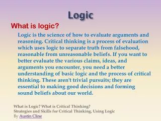
Logic. What is logic?. Logic is an “algebra” for manipulating only two values: true ( T ) and false ( F ) Nevertheless, logic can be quite challenging This talk will cover: Propositional logic--the simplest kind

Logic
E N D
Presentation Transcript
What is logic? • Logic is an “algebra” for manipulating only two values: true (T) and false (F) • Nevertheless, logic can be quite challenging • This talk will cover: • Propositional logic--the simplest kind • Predicate logic (a.k.a. predicate calculus)--an extension of propositional logic • Resolution theory--a general way of doing proofs in predicate logic • Possibly: Conversion to clause form • Possibly: Other logics (just to make you aware that they exist)
Propositional logic • Propositional logic consists of: • The logical values trueandfalse(TandF) • Propositions: “Sentences,” which • Are atomic (that is, they must be treated as indivisible units, with no internal structure), and • Have a single logical value, either true or false • Operators, both unary and binary; when applied to logical values, yield logical values • The usual operators are and, or, not, and implies
Truth tables • Logic, like arithmetic, has operators, which apply to one, two, or more values (operands) • A truth table lists the results for each possible arrangement of operands • Order is important: x op y may or may not give the same result as y op x • The rows in a truth table list all possible sequences of truth values for n operands, and specify a result for each sequence • Hence, there are 2n rows in a truth table for n operands
There are four possible unary operators: Only the last of these (negation) is widely used (and has a symbol,¬ ,for the operation Unary operators
There are sixteen possible binary operators: All these operators have names, but I haven’t tried to fit them in Only a few of these operators are normally used in logic Binary operators
Notice in particular that material implication () only approximately means the same as the English word “implies” All the other operators can be constructed from a combination of these (along with unary not, ¬) Useful binary operators • Here are the binary operators that are traditionally used:
All logical expressions can be computed with some combination of and (), or (), and not () operators For example, logical implication can be computed this way: Notice that X Y is equivalent to X Y Logical expressions
Exclusive or (xor) is true if exactly one of its operands is true Notice that (XY)(XY)is equivalent to X xor Y Another example
Worlds • A world is a collection of prepositions and logical expressions relating those prepositions • Example: • Propositions: JohnLovesMary, MaryIsFemale, MaryIsRich • Expressions:MaryIsFemale MaryIsRich JohnLovesMary • A proposition “says something” about the world, but since it is atomic (you can’t look inside it to see component parts), propositions tend to be very specialized and inflexible
Models A model is an assignment of a truth value to each proposition, for example: • JohnLovesMary: T, MaryIsFemale: T, MaryIsRich: F • An expression is satisfiable if there is a model for which the expression is true • For example, the above model satisfies the expressionMaryIsFemale MaryIsRich JohnLovesMary • An expression is valid if it is satisfied by every model • This expression is not valid:MaryIsFemale MaryIsRich JohnLovesMarybecause it is not satisfied by this model:JohnLovesMary: F, MaryIsFemale: T, MaryIsRich: T • But this expression is valid:MaryIsFemale MaryIsRich MaryIsFemale
From aima.eecs.berkeley.edu/slides-ppt, chs 7-9 Inference rules in propositional logic • Here are just a few of the rules you can apply when reasoning in propositional logic:
Implication elimination • A particularly important rule allows you to get rid of the implication operator, : • X Y X Y • We will use this later on as a necessary tool for simplifying logical expressions • The symbol means “is logically equivalent to”
Conjunction elimination • Another important rule for simplifying logical expressions allows you to get rid of the conjunction (and) operator, : • This rule simply says that if you have an and operator at the top level of a fact (logical expression), you can break the expression up into two separate facts: • MaryIsFemale MaryIsRich • becomes: • MaryIsFemale • MaryIsRich
Inference by computer • To do inference (reasoning) by computer is basically a search process, taking logical expressions and applying inference rules to them • Which logical expressions to use? • Which inference rules to apply? • Usually you are trying to “prove” some particular statement • Example: • it_is_raining it_is_sunny • it_is_sunny I_stay_dry • it_is_rainy I_take_umbrella • I_take_umbrella I_stay_dry • To prove: I_stay_dry
Forward and backward reasoning • Situation: You have a collection of logical expressions (premises), and you are trying to prove some additional logical expression (the conclusion) • You can: • Do forward reasoning: Start applying inference rules to the logical expressions you have, and stop if one of your results is the conclusion you want • Do backward reasoning: Start from the conclusion you want, and try to choose inference rules that will get you back to the logical expressions you have • With the tools we have discussed so far, neither is feasible
Example • Given: • it_is_raining it_is_sunny • it_is_sunny I_stay_dry • it_is_raining I_take_umbrella • I_take_umbrella I_stay_dry • You can conclude: • it_is_sunny it_is_raining • I_take_umbrella it_is_sunny • I_stay_dry I_take_umbrella • Etc., etc. ... there are just too many things you can conclude!
Predicate calculus • Predicate calculus is also known as “First Order Logic” (FOL) • Predicate calculus includes: • All of propositional logic • Logical values true, false • Variables x, y, a, b,... • Connectives , , , , • Constants KingJohn, 2, Villanova,... • Predicates Brother, >,... • Functions Sqrt, MotherOf,... • Quantifiers ,
Constants, functions, and predicates • A constant represents a “thing”--it has no truth value, and it does not occur “bare” in a logical expression • Examples: DavidMatuszek, 5, Earth, goodIdea • Given zero or more arguments, a function produces a constant as its value: • Examples: motherOf(DavidMatuszek), add(2, 2), thisPlanet() • A predicate is like a function, but produces a truth value • Examples: greatInstructor(DavidMatuszek), isPlanet(Earth), greater(3, add(2, 2))
Universal quantification • The universal quantifier, , is read as “for each” or “for every” • Example: x, x2 0 (for all x, x2 is greater than or equal to zero) • Typically, is the main connective with : x, at(x,Villanova) smart(x) means “Everyone at Villanova is smart” • Common mistake: using as the main connective with : x, at(x,Villanova) smart(x) means “Everyone is at Villanova and everyone is smart” • If there are no values satisfying the condition, the result is true • Example: x, isPersonFromMars(x) smart(x) is true
Existential quantification • The existential quantifier, , is read “for some” or “there exists” • Example: x, x2 < 0 (there exists an x such that x2 is less than zero) • Typically, is the main connective with : x, at(x,Villanova) smart(x) means “There is someone who is at Villanova and is smart” • Common mistake: using as the main connective with : x, at(x,Villanova) smart(x) This is true if there is someone at Villanova who is smart... ...but it is also true if there is someone who is not at Villanova By the rules of material implication, the result of F T is T
Properties of quantifiers • x yis the same asyx • x y is the same asyx • x y is not the same as yx • x y Loves(x,y) • “There is a person who loves everyone in the world” • More exactly: x y (person(x) person(y) Loves(x,y)) • yx Loves(x,y) • “Everyone in the world is loved by at least one person” • Quantifier duality: each can be expressed using the other • x Likes(x,IceCream) x Likes(x,IceCream) • x Likes(x,Broccoli) xLikes(x,Broccoli) From aima.eecs.berkeley.edu/slides-ppt, chs 7-9
Parentheses • Parentheses are often used with quantifiers • Unfortunately, everyone uses them differently, so don’t be upset at any usage you see • Examples: • (x) person(x) likes(x,iceCream) • (x) (person(x) likes(x,iceCream)) • (x) [ person(x) likes(x,iceCream) ] • x, person(x) likes(x,iceCream) • x (person(x) likes(x,iceCream)) • I prefer parentheses that show the scope of the quantifier • x (x > 0) x (x < 0)
More rules • Now there are numerous additional rules we can apply! • Here are two exceptionally important rules: • x, p(x) x, p(x)“If not every x satisfies p(x), then there exists a x that does not satisfy p(x)” • x, p(x) x, p(x)“If there does not exist an x that satisfies p(x), then all x do not satisfy p(x)” • In any case, the search space is just too large to be feasible • This was the case until 1970, when J. Robinson discovered resolution
Interlude: Definitions • syntax: defines the formal structure of sentences • semantics: determines the truth of sentences wrt (with respect to) models • entailment: one statement entails another if the truth of the first means that the second must also be true • inference: deriving sentences from other sentences • soundness: derivations produce only entailed sentences • completeness: derivations can produce all entailed sentences
Logic by computer was infeasible • Why is logic so hard? • You start with a large collection of facts (predicates) • You start with a large collection of possible transformations (rules) • Some of these rules apply to a single fact to yield a new fact • Some of these rules apply to a pair of facts to yield a new fact • So at every step you must: • Choose some rule to apply • Choose one or two facts to which you might be able to apply the rule • If there are n facts • There are n potential ways to apply a single-operand rule • There are n * (n - 1) potential ways to apply a two-operand rule • Add the new fact to your ever-expanding fact base • The search space is huge!
The magic of resolution • Here’s how resolution works: • You transform each of your facts into a particular form, called a clause (this is the tricky part) • You apply a single rule, the resolution principle, to a pair of clauses • Clauses are closed with respect to resolution--that is, when you resolve two clauses, you get a new clause • You add the new clause to your fact base • So the number of facts you have grows linearly • You still have to choose a pair of facts to resolve • You never have to choose a rule, because there’s only one
The fact base • A fact base is a collection of “facts,” expressed in predicate calculus, that are presumed to be true (valid) • These facts are implicitly “anded” together • Example fact base: • seafood(X) likes(John, X) (where X is a variable) • seafood(shrimp) • pasta(X) likes(Mary, X) (where X is a different variable) • pasta(spaghetti) • That is, • (seafood(X) likes(John, X)) seafood(shrimp) (pasta(Y) likes(Mary, Y)) pasta(spaghetti) • Notice that we had to change some Xs to Ys • The scope of a variable is the single fact in which it occurs
Clause form • A clause is a disjunction ("or") of zero or more literals, some or all of which may be negated • Example:sinks(X) dissolves(X, water) ¬denser(X, water) • Notice that clauses use only “or” and “not”—they do not use “and,” “implies,” or either of the quantifiers “for all” or “there exists” • The impressive part is that any predicate calculus expression can be put into clause form • Existential quantifiers, , are the trickiest ones
Unification • From the pair of facts (not yet clauses, just facts): • seafood(X) likes(John, X) (where X is a variable) • seafood(shrimp) • We ought to be able to conclude • likes(John, shrimp) • We can do this by unifying the variable X with the constant shrimp • This is the same “unification” as is done in Prolog • This unification turnsseafood(X) likes(John, X) intoseafood(shrimp) likes(John, shrimp) • Together with the given fact seafood(shrimp), the final deductive step is easy
The resolution principle • Here it is: • From X someLiteralsand X someOtherLiterals ----------------------------------------------conclude: someLiterals someOtherLiterals • That’s all there is to it! • Example: • broke(Bob) well-fed(Bob)¬broke(Bob) ¬hungry(Bob)--------------------------------------well-fed(Bob) ¬hungry(Bob)
A common error • You can only do one resolution at a time • Example: • broke(Bob) well-fed(Bob) happy(Bob)¬broke(Bob) ¬hungry(Bob) ∨ ¬happy(Bob) • You can resolve on broke to get: • well-fed(Bob) happy(Bob) ¬hungry(Bob) ¬happy(Bob) T • Or you can resolve on happy to get: • broke(Bob) well-fed(Bob) ¬broke(Bob) ¬hungry(Bob) T • Note that both legal resolutions yield a tautology (a trivially true statement, containing X ¬X), which is correct but useless • But you cannot resolve on both at once to get: • well-fed(Bob) ¬hungry(Bob)
Contradiction • A special case occurs when the result of a resolution (the resolvent) is empty, or “NIL” • Example: • hungry(Bob)¬hungry(Bob)----------------NIL • In this case, the fact base is inconsistent • This will turn out to be a very useful observation in doing resolution theorem proving
A first example • “Everywhere that John goes, Rover goes. John is at school.” • at(John, X) at(Rover, X) (not yet in clause form) • at(John, school) (already in clause form) • We use implication elimination to change the first of these into clause form: • at(John, X) at(Rover, X) • at(John, school) • We can resolve these on at(-, -), but to do so we have to unify X with school; this gives: • at(Rover, school)
Refutation resolution • The previous example was easy because it had very few clauses • When we have a lot of clauses, we want to focus our search on the thing we would like to prove • We can do this as follows: • Assume that our fact base is consistent (we can’t derive NIL) • Add the negation of the thing we want to prove to the fact base • Show that the fact base is now inconsistent • Conclude the thing we want to prove
Example of refutation resolution • “Everywhere that John goes, Rover goes. John is at school. Prove that Rover is at school.” • at(John, X) at(Rover, X) • at(John, school) • at(Rover, school) (this is the added clause) • Resolve #1 and #3: • at(John, X) • Resolve #2 and #4: • NIL • Conclude the negation of the added clause: at(Rover, school) • This seems a roundabout approach for such a simple example, but it works well for larger problems
Start with: it_is_raining it_is_sunny it_is_sunny I_stay_dry it_is_raining I_take_umbrella I_take_umbrella I_stay_dry Convert to clause form: it_is_raining it_is_sunny it_is_sunny I_stay_dry it_is_raining I_take_umbrella I_take_umbrella I_stay_dry Prove that I stay dry: I_stay_dry Proof: (5, 2) it_is_sunny (6, 1) it_is_raining (5, 4) I_take_umbrella (8, 3) it_is_raining (9, 7) NIL Therefore, (I_stay_dry) I_stay_dry A second example
Conversion to clause form A nine-step process Reference: Artificial Intelligence, by Elaine Rich and Kevin Knight
Running example • All Romans who know Marcus either hate Caesar or think that anyone who hates anyone is crazy • x, [ Roman(x) know(x, Marcus) ] [ hate(x, Caesar) (y, z, hate(y, z) thinkCrazy(x, y))]
Step 1: Eliminate implications • Use the fact that x y is equivalent to x y • x, [ Roman(x) know(x, Marcus) ] [ hate(x, Caesar) (y, z, hate(y, z) thinkCrazy(x, y))] • x, [ Roman(x) know(x, Marcus) ] [hate(x, Caesar) (y, (z, hate(y, z) thinkCrazy(x, y))]
Step 2: Reduce the scope of • Reduce the scope of negation to a single term, using: • (p) p • (a b) (a b) • (a b) (a b) • x, p(x) x, p(x) • x, p(x) x, p(x) • x, [ Roman(x) know(x, Marcus) ] [hate(x, Caesar) (y, (z, hate(y, z) thinkCrazy(x, y))] • x, [ Roman(x) know(x, Marcus) ] [hate(x, Caesar) (y, z, hate(y, z) thinkCrazy(x, y))]
Step 3: Standardize variables apart • x, P(x) x, Q(x) becomes x, P(x) y, Q(y) • This is just to keep the scopes of variables from getting confused • Not necessary in our running example
Step 4: Move quantifiers • Move all quantifiers to the left, without changing their relative positions • x, [ Roman(x) know(x, Marcus) ] [hate(x, Caesar) (y, z, hate(y, z) thinkCrazy(x, y)] • x, y, z,[ Roman(x) know(x, Marcus) ] [hate(x, Caesar) (hate(y, z) thinkCrazy(x, y))]
Step 5: Eliminate existential quantifiers • We do this by introducing Skolem functions: • If x, p(x) then just pick one; call it x’ • If the existential quantifier is under control of a universal quantifier, then the picked value has to be a function of the universally quantified variable: • If x, y, p(x, y) then x, p(x, y(x)) • Not necessary in our running example
Step 6: Drop the prefix (quantifiers) • x, y, z,[ Roman(x) know(x, Marcus) ] [hate(x, Caesar) (hate(y, z) thinkCrazy(x, y))] • At this point, all the quantifiers are universal quantifiers • We can just take it for granted that all variables are universally quantified • [ Roman(x) know(x, Marcus) ] [hate(x, Caesar) (hate(y, z) thinkCrazy(x, y))]
Step 7: Create a conjunction of disjuncts • [ Roman(x) know(x, Marcus) ] [hate(x, Caesar) (hate(y, z) thinkCrazy(x, y))]becomes Roman(x) know(x, Marcus) hate(x, Caesar) hate(y, z) thinkCrazy(x, y)