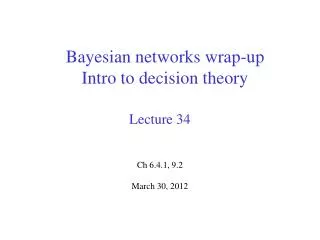
Bayesian networks wrap-up Intro to decision theory
520 likes | 638 Vues
Bayesian networks wrap-up Intro to decision theory. Lecture 35 Ch 9.2 April 2, 2012. Announcements (1) . Remember to fill out the online Teaching Evaluations! You should have received various email messages about them Secure, confidential, mobile access

Bayesian networks wrap-up Intro to decision theory
E N D
Presentation Transcript
Bayesian networks wrap-up Intro to decision theory Lecture 35 Ch 9.2 April 2, 2012
Announcements (1) • Remember to fill out the online Teaching Evaluations! • You should have received various email messages about them • Secure, confidential, mobile access • Your feedback is important! • Evaluations close at 11pm on April 10th, 2011 • Before exam, but instructors can’t see results until after we submit grades • Take a few minutes and visit https://eval.olt.ubc.ca/science
Announcements (1) • Final exam • Friday, April 13t, 8:30 – 11am in DMP 310 • Same general format as midterm (~50 % short questions) • List from which I will draw these questions will be on WebCT • Will also post other practice problems • How to study? • Practice exercises, assignments, short questions, lecture notes, book, … • Use TA and my office hours • extra office hours for next week, also posted on class schedule
Lecture Overview • Recap Lecture 34 and Bayesian networks wrap up • Decisions under Uncertainty • Intro • Utility and expected utility • Single-stage decision problems • Decision networks (time permitting)
6. Normalize by dividing the resulting factor f(Y) by The variable elimination algorithm, The JPD of a Bayesian network is • Construct a factor for each conditional probability. • For each factor, assign the observed variables E to their observed values. • Given an elimination ordering, decompose sum of products • Sum out all variables Zinot involved in the query (one a time) • Multiply factors containing Zi • Then marginalize out Zifrom the product • Multiply the remaining factors (which only involve Y ) To compute P(Y=yi| E = e)
VE and conditional independence • Before running VE, we can prune all variables Z that are conditionally independent of the query Y given evidence E: Z ╨ Y | E • They cannot change the belief over Y given E! • Example: which variables can we prune for the query P(G=g| C=c1, F=f1, H=h1) ? • A, B, and D. Both paths from these nodes to G are blocked • F is observed node in chain structure • C is an observed common parent • Thus, we only need to consider this subnetwork
One last trick • We can also prune unobserved leaf nodes, recursively • Since they are unobserved and not predecessors of the query nodes, they cannot influence the posterior probability of the query nodes • E.g., which nodes can we prune if the query is P(A)? • Recursively prune unobserved leaf nodes: • we can prune all nodes other than A !
Complexity of Variable Elimination (VE) • A factor over n binary variables has to store 2n numbers • The initial factors are typically quite small • But variable elimination constructs larger factors by multiplying factors together • The complexity of VE is exponential in the maximum number of variables in any factor during its execution • This number is called the treewidth of a graph (along an ordering) • Elimination ordering influences treewidth, but finding the best ordering is NP complete • Heuristics work well in practice (e.g. least connected variables first)
Learning Goals For VE • Variable elimination • Understating factors and their operations • Carry out variable elimination by using factors and the related operations • Use techniques to simplify variable elimination
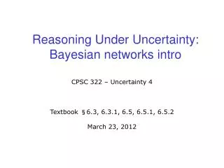
Big picture: Reasoning Under Uncertainty Probability Theory Bayesian Networks & Variable Elimination Dynamic Bayesian Networks Hidden Markov Models & Filtering Monitoring(e.g. credit card fraud detection) Bioinformatics Motion Tracking,Missile Tracking, etc Natural Language Processing Diagnostic systems(e.g. medicine) Email spam filters
One Realistic BN: Liver DiagnosisSource: Onisko et al., 1999 ~60 nodes, max 4 parents per node
Realistic BNet: Student TracingSource: ConatiGertner and VanLehn 2002 • Andes Tutor for Physics captures student problem solving actions • Sends them as evidence to a Bnet that assesses student knowledge of relevant physics principles • Based on the network prediction, Andes provides interactive help to the student • Used routinely at the US Naval Academy as homework aid
Where are we? Representation • Environment Reasoning Technique Stochastic Deterministic Problem Type This concludes the module on answering queries in stochastic environments Arc Consistency Constraint Satisfaction Vars + Constraints Search Static Belief Nets Logics Variable Elimination Query Search Decision Nets Sequential STRIPS Variable Elimination Planning Search
What’s Next? Representation • Environment Reasoning Technique Stochastic Deterministic Problem Type Arc Consistency Now we will look at acting in stochastic environments Constraint Satisfaction Vars + Constraints Search Static Belief Nets Logics Variable Elimination Query Search Decision Nets Sequential STRIPS Variable Elimination Planning Search
Lecture Overview • Recap Lecture 34 and Bayesian networks wrap up • Decisions under Uncertainty • Intro • Utility and expected utility • Single-stage decision problems • Decision networks (time permitting)
Decisions Under Uncertainty: Intro • An agent's decision will depend on • What actions are available • What beliefs the agent has • Which goals the agent has • Differences between deterministic and stochastic setting • Obvious difference in representation: need to represent our uncertain beliefs • Actions will be pretty straightforward: represented as decision variables • Goals will be interesting: we'll move from all-or-nothing goals to a richer notion: • rating how happy the agent is in different situations. • Putting these together, we'll extend Bayesian Networks to make a new representation called Decision Networks
Delivery Robot Example • Robot needs to reach a certain room • Robot can go • the short way - faster but with more obstacles, thus more prone to accidents that can damage the robot and prevent it from reaching the room • the long way - slower but less prone to accident • Which way to go? Is it more important for the robot to arrive fast, or to minimize the risk of damage? • The Robot can choose to wear pads to protect itself in case of accident, or not to wear them. Pads slow it down • Again, there is a tradeoff between reducing risk of damage and arriving fast • Possible outcomes • No pad, no accident • Pad, no accident • Pad, Accident • No pad, accident
Next • We’ll see how to represent and reason about situations of this nature by using • Probability to measure the uncertainty in actions outcome • Utility to measure agent’s preferences over the various outcomes • Combined in a measure of expected utility that can be used to identify the action with the best expected outcome • Best that an intelligent agent can do when it needs to act in a stochastic environment
Decision Tree for the Delivery Robot Example • Decision variable 1: the robot can choose to wear pads • Yes: protection against accidents, but extra weight • No: fast, but no protection • Decision variable 2: the robot can choose the way • Short way: quick, but higher chance of accident • Long way: safe, but slow • Random variable: is there an accident? Agent decides Chance decides
Delivery Robot Example • Decision variable 1: the robot can choose to wear pads • Yes: protection against accidents, but extra weight • No: fast, but no protection • Decision variable 2: the robot can choose the way • Short way: quick, but higher chance of accident • Long way: safe, but slow • Random variable: is there an accident? Agent decides Chance decides
Possible worlds and decision variables • A possible world specifies a value for each random variable and each decision variable • For each assignment of values to all decision variables • the probabilities of the worlds satisfying that assignment sum to 1. 0.2 0.8
Possible worlds and decision variables • A possible world specifies a value for each random variable and each decision variable • For each assignment of values to all decision variables • the probabilities of the worlds satisfying that assignment sum to 1. 0.2 0.8 0.01 0.99
Possible worlds and decision variables • A possible world specifies a value for each random variable and each decision variable • For each assignment of values to all decision variables • the probabilities of the worlds satisfying that assignment sum to 1. 0.2 0.8 0.01 0.99 0.2 0.8
Possible worlds and decision variables • A possible world specifies a value for each random variable and each decision variable • For each assignment of values to all decision variables • the probabilities of the worlds satisfying that assignment sum to 1. 0.2 0.8 0.01 0.99 0.2 0.8 0.01 0.99
Lecture Overview • Recap Lecture 34 and Bayesian networks wrap up • Decisions under Uncertainty • Intro • Utility and expected utility • Single-stage decision problems • Decision networks (time permitting)
Utility • Utility: a measure of desirability of possible worlds to an agent • Let U be a real-valued function such that U(w) represents an agent's degree of preference for world w • Expressed by a number in [0,100] • Simple goals can still be specified • Worlds that satisfy the goal have utility 100 • Other worlds have utility 0 • Utilities can be more complicated • For example, in the robot delivery domains, they could involve • Reached the target room? • Time taken • Amount of damage • Energy left
Utility for the Robot Example • Which would be a reasonable utility function for our robot? • Which are the best and worst scenarios? probability Utility 0.2 0.8 0.01 0.99 0.2 0.8 0.01 0.99
Utility for the Robot Example • Now, how do we combine utility and probability to decide what to do? probability Utility 0.2 35 35 95 0.8 35 30 0.01 75 0.99 0.2 35 3 100 0.8 35 0 0.01 80 0.99
Optimal decisions: combining Utility and Probability • Each set of decisions defines a probability distribution over possible outcomes • Each outcome has a utility • For each set of decisions, we need to know their expected utility • the value for the agent of achieving a certain probability distribution over outcomes (possible worlds) 0.2 35 95 0.8 value of this scenario? • The expected utility of a set of decisions is obtained by • weighting the utility of the relevant possible worlds by their probability. • We want to find the decision with maximum expected utility
Expected utility of a decision • The expected utility of decision D = di is • What is the expected utility of Wearpads=yes, Way=short ? E(U | D = di) =w╞ (D = di)P(w) U(w) probability Utility E[U|D] 0.2 35 35 95 0.8 30 35 0.01 75 0.99 0.2 35 3 100 0.8 35 0 0.01 80 0.99
Expected utility of a decision • The expected utility of decision D = di is • What is the expected utility of Wearpads=yes, Way=short ? • 0.2 * 35 + 0.8 * 95 = 83 E(U | D = di) =w╞ (D = di)P(w) U(w) Conditional probability Utility E[U|D] 0.2 35 35 83 95 0.8 35 30 0.01 74.55 75 0.99 0.2 35 3 80.6 100 0.8 35 0 0.01 79.2 80 0.99
Lecture Overview • Recap Lecture 34 and Bayesian networks wrap up • Decisions under Uncertainty • Intro • Utility and expected utility • Single-stage decision problems • Decision networks (time permitting)
Single Action vs. Sequence of Actions • Single Action (aka One-Off Decisions) • One or more primitive decisions that can be treated as a single macro decision to be made before acting • E.g., “WearPads” and “WhichWay” can be combined into macro decision (WearPads, WhichWay) with domain {yes,no} × {long, short} • Sequence of Actions (Sequential Decisions) • Repeat: • make observations • decide on an action • carry out the action • Agent has to take actions not knowing what the future brings • This is fundamentally different from everything we’ve seen so far • Planning was sequential, but we still could still think first and then act
Optimal single-stage decision • Given a single (macro) decision variable D • the agent can choose D=difor any value di dom(D)
What is the optimal decision in the example? Conditional probability (Wear pads, short way) Utility E[U|D] (Wear pads, long way) 0.2 35 35 (No pads, short way) 83 95 0.8 (No pads, long way) 30 35 0.01 74.55 75 0.99 0.2 35 3 80.6 100 0.8 35 0 0.01 79.2 80 0.99
Optimal decision in robot delivery example Best decision: (wear pads, short way) Conditional probability Utility E[U|D] 0.2 35 35 83 95 0.8 30 35 0.01 74.55 75 0.99 0.2 35 3 80.6 100 0.8 35 0 0.01 79.2 80 0.99
Learning Goals For Today’s Class • Next time: • Decision networks for one-off decisions • Variable Elimination for one-off decision • Sequentialdecisions • Define a Utility Function on possible worlds • Define and compute optimal one-off decisions
Lecture Overview • Recap Lecture 34 and Bayesian networks wrap up • Decisions under Uncertainty • Intro • Utility and expected utility • Single-stage decision problems • Decision networks for single-stage decision problems (time permitting)
Single-Stage decision networks • Extend belief networks with: • Decision nodes, that the agent chooses the value for • Parents: only other decision nodes allowed • Domain is the set of possible actions • Drawn as a rectangle • Exactly one utility node • Parents: all random & decision variables on which the utility depends • Does not have a domain • Drawn as a diamond • Explicitly shows dependencies • E.g., which variables affect the probability of an accident?
Types of nodes in decision networks • A random variable is drawn as an ellipse. • Arcs into the node represent probabilistic dependence • As in Bayesian networks: a random variable is conditionally independent of its non-descendants given its parents • A decision variable is drawn as an rectangle. • Arcs into the node represent information available when the decision is made • A utility node is drawn as a diamond. • Arcs into the node represent variables that the utility depends on. • Specifies a utility for each instantiation of its parents
Example Decision Network Decision nodes do not have an associated table. The utility node does not have a domain.
Lecture Overview • Recap Lecture 34 and Bayesian networks wrap up • Decisions under Uncertainty • Intro • Utility and expected utility • Single-stage decision problems • Decision networks for single-stage decision problems (time permitting) • Variable Elimination for single stage decision networks
Computing the optimal decision: we can use VE • Denote • the random variables as X1, …, Xn • the decision variables as D • the parents of node N as pa(N) • To find the optimal decision we can use VE: • Create a factor for each conditional probability and for the utility • Sum out all random variables, one at a time • This creates a factor on D that gives the expected utility for each di • Choose the di with the maximum value in the factor
VE Example: Step 1, create initial factors f1(A,W) Abbreviations: W = Which WayP = Wear PadsA = Accident f2(A,W,P)
VE example: step 2, sum out A Step 2a: compute product f(A,W,P) = f1(A,W) × f2(A,W,P) f(A=a,P=p,W=w) = f1(A=a,W=w) × f2(A=a,W=w,P=p) 0.99 * 30 0.01 * 80 0.99 * 80 0.8 * 30
VE example: step 2, sum out A Step 2a: compute product f(A,W,P) = f1(A,W) × f2(A,W,P) f(A=a,P=p,W=w) = f1(A=a,W=w) × f2(A=a,W=w,P=p)
VE example: step 2, sum out A Step 2b: sum A out of the product f(A,W,P): 0.2*35 + 0.2*0.3 0.2*35 + 0.8*95 0.99*80 + 0.8*95 0.8 * 95 + 0.8*100
VE example: step 2, sum out A Step 2b: sum A out of the product f(A,W,P):
VE example: step 2, sum out A Step 2b: sum A out of the product f(A,W,P):
VE example: step 3, choose decision with max E(U) The final factor encodes the expected utility of each decision • Thus, taking the short way but wearing pads is the best choice, with an expected utility of 83 Step 2b: sum A out of the product f(A,W,P):