Bayesian Decision Theory

1. Bayesian Decision Theory

2. Pattern Classification Bayesian Decision Theory

3. Retrospective Bayesian Multimodal Perception by J. F. Fereira Bayes' theorem - Bayes rule Knowledge of past behavior and state form prediction of current state Non-Gaussian likelihood functions Multimodal Sensing in human perception

4. Retrospective distribution of object position unknown => flat Noise in each modality is independent bimodal posterior distribution = product of the unimodal distributions Simplification: Probability distributions are Gaussian

5. 1. Introduction to Pattern Recognition Example: “Sorting incoming Fish on a conveyor according to species using optical sensing”

6. 1. Introduction to Pattern Recognition Example: Fish Classifier Selecting length feature Selecting lightness feature

7. 1. Introduction to Pattern Recognition Best performance but complicated classifier – will not perform well with novel patterns Search for the optimal tradeoff between performance on the training set and simplicity Selecting two features and defining a simple straight line as decision boundary Example: Fish Classifier

8. 1. Introduction to Pattern Recognition decision Pattern Recognition System post-processing Invariant Features Translation Rotation Scale Occlusion Projective Distortion Rate Deformation Feature Selection Noise Missing Features Error Rate Risk Context Multiple Classifiers classification feature extraction segmentation sensing input

9. 1. Introduction to Pattern Recognition start Design Cycle collect data Prior Knowledge Overfitting choose features choose model train classifier evaluate classifier end

10. 2. Continouos Features State of nature Finite set of c states of nature (‘categories’) {1, … , c} PriorP(j) If the state of nature is finite: Decision rule (for c =2): Decide 1 if P(1) > P(2); otherwise decide 2

11. 2. Continouos Features Feature vector x : x d the feature space x is (for d=1) a continuous random variable x Class(State)-conditional probability density function: p(x| j) expresses the distribution of x depending on the state of nature

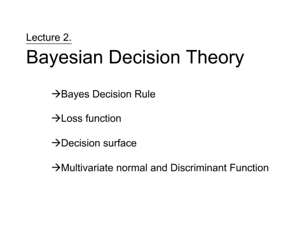
12. 2. Continouos Features Bayes formula (Posterior) Evidence Bayes Decision rule (for c =2): Decide 1 if P(1 | x)> P(2 | x); otherwise decide 2 Bayes Decision rule (expressed in terms of Priors): Decide 1 if p(x|1)P(1)> p(x|2)P(2); otherwise decide 2

13. 2. Continouos Features Bayes Risk Conditional Risk We can minimize our expected loss by selecting the action that minimizes the conditional risk. Two-Category Classification Decide 1 if (21-11)P(1 | x)> (12-22)P(2 | x); otherwise decide 2 This Bayes decision procedure provides the optimal performance

14. Discrete Features Feature vector x can assume m discrete values Posterior Probabilities rather than probability densities. Evidence Risk Bayes decision rule To minimize the overall risk, select the action I for which R(i|x) is minimum

15. Discrete Features Example: Independent Binary Features 2 category problem Feature vector x = {x1, …, xd}T where xi = {0;1}

16. variable node P(a) link parents (of C) children (of E) Bayesian Belief Networks Represents knowledge about a distribution. Knowledge: Statistical Dependencies – Causal Relations among the component variables Knowledge from e.g. structural information Graphical representation: Bayesian Belief Nets

17. Bayesian Belief Networks Applying Bayes rule to determine the probability of any configuration of variables in the joint distribution. Discrete Case: Discrete number of possible values A (e.g. 2: a={a1, a2} and continues-valued probabilities =1 Conditional Probability Table =1 =1

18. Bayesian Belief Networks Determining the probabilities of the variables P(a) P(b|a) P(c|b) P(d|c) A B C D E.g.: Probability distribution over d1, d2, … at D Summing the full joint distribution P(a,b,c,d) over all variables other than d independance simple split simple interpretation P(b) P(c) P(d) Probability of a particular value of D

19. Bayesian Belief Networks Give the values of some variables (evidence e) … and search to determine some particular configuration of other variables x

20. Bayesian Belief Networks Example: Belief Network for Fish Ex.2 Classify the fish: Known: Fish is light (c1) and caught in the south Atlantic (b2). Unknown: Time of year (a), thickness (d) As usual: Compute P(x1 salmon) and P(x2 sea bass) Decide for the minimum expected classification error In this case D does not affect our results

21. Bayesian Belief Networks Example: Belief Network for Fish

22. Bayesian Belief Networks Example: Belief Network for Fish After normalization: And if the dependency relation is unknown? naïve Bayes – idiot Bayes Features are conditionally independant

23. Compound Bayesian Decision Theory Consecutive ’s not statistically independent => exploit dependence => improved performance Wait for n states to emerge and make all n decisions jointly = compound decision problem States of nature = ((1), … , (n))T taking one of c values {1, … , c} PriorP() for n states of nature Feature matrix X : =(x1, …, xn) xi obtained when state of nature was i n observations

24. Compound Bayesian Decision Theory Define loss matrix for the compound decision problem. Seek decision rule the minimizes the compound risk (optimal procedure) Assumption: Correct = no loss Errors = equally costly => simply calculate P(|X) for all  and select  for which P(.) is maximum. practice: calculate P(|X) is time expensive assumption: xi depends only on (i) not on other x or  Conditional probability density function: p(X|) for X given the true set of  Posterior joint density

25. Obrigado!

26. Annex

27. Book: Pattern Cl. PrefaceCh 1: Introduction Ch 2: Bayesian Decision Theory Ch 3: Maximum Likelihood and Bayesian Estimation Ch 4: Nonparametric Techniques Ch 5: Linear Discriminant Functions Ch 6: Multilayer Neural Networks Ch 7: Stochastic Methods Ch 8: Nonmetric Methods Ch 9: Algorithm-Independent Machine Learning Ch 10: Unsupervised Learning and Clustering App A: Mathematical Foundations

28. Book: Principles of ...

29. Book: Artificial ... Preface Part I Artificial Intelligence Part II Problem Solving Part III Knowledge and Reasoning Part IV Planning Part V Uncertain Knowledge and Reasoning Part VI Learning Part VII Communicating, Perceiving, and Acting Part VIII Conclusions

30. Book: Bayesian ... Preface xix Part I: Fundamentals of Bayesian Inference 1 1 Background 3 2 Single-parameter models 33 3 Introduction to multiparameter models 73 4 Large-sample inference and frequency properties of Bayesian inference 101 Part II: Fundamentals of Bayesian Data Analysis 115 5 Hierarchical models 117 6 Model checking and improvement 157 7 Modeling accounting for data collection 197 8 Connections and challenges 247 9 General advice 259 Part III: Advanced Computation 273 10 Overview of computation 275 11 Posterior simulation 283 12 Approximations based on posterior modes 311 13 Special topics in computation 335 Part IV: Regression Models 351 14 Introduction to regression models 353 15 Hierarchical linear models 389 16 Generalized linear models 415 17 Models for robust inference 443 18 Mixture models 463 19 Multivariate models 481 20 Nonlinear models 497 21 Models for missing data 517 22 Decision analysis 541 Appendixes 571

31. Book: Classification ... Preface. Foreword. 1. Introduction. 2. Detection and Classification. 3. Parameter Estimation. 4. State Estimation. 5. Supervised Learning. 6. Feature Extraction and Selection. 7. Unsupervised Learning. 8. State Estimation in Practice. 9. Worked Out Examples. Appendix

32. Images

33. 2. Simple Example Ten types of gestures: 1. Big circle 2. Small circle 3. Vertical Line 4. Horizontal Line 5. Pointing North-West 6. Pointing West 7. Talk louder 8. Talk more quiet 9. Wave Bye-Bye 10. I am hungry Designing a simple classifier for gesture recognition. The observer tries to predict which gesture might be performed next. The sequence of gestures appears to be random. We assume that there is some a priori probability (i.e. prior) P(1) that the next gesture is ‘Big Circle’, P(2) that the next gesture is ‘Small Circle’, etc. If the gesture lexicon is finite: State of nature   Type of gesture (1 … 10)

34. Missing and noisy features Missing Features: Example: x1 is missing measured value of x2 is x^2 mean x1 points to omega 3 but omega2 better decision