Mastering Data Visualization in R with Graphics Functions
200 likes | 228 Vues
Learn to create bar charts, pie charts, histograms, box plots, and scatter plots in R with ease. Explore different plot types and customize visualizations to represent data effectively using R's graphics packages. Dive into code examples and practice creating various graphs in R.

Mastering Data Visualization in R with Graphics Functions
E N D
Presentation Transcript
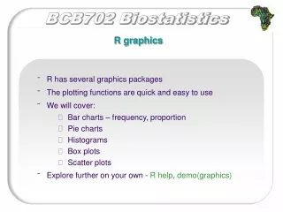
R graphics • R has several graphics packages • The plotting functions are quick and easy to use • We will cover: • Bar charts – frequency, proportion • Pie charts • Histograms • Box plots • Scatter plots • Explore further on your own - R help, demo(graphics)
Bar charts • A bar chart draws a bar with a height proportional to the count in the table • The height could be given by the frequency, or the proportion, where the graph will look the same, but the scales may be different • Use scan() to read in the data from a file or by typing • Try ?scan for more information • Usage is simple: type in the data. It stops adding data when you enter a blank row
Bar charts Example: • Suppose, a group of 25 animals are surveyed for their feeding preference. The categories are (1) grass, (2) shrubs, (3) trees and (4) fruit. The raw data is 3 4 1 1 3 4 3 3 1 3 2 1 2 1 2 3 2 3 1 1 1 1 4 3 1 • Let's make a barplot of both frequencies and proportions…
Frequency Bar chart - frequency Example: Feeding preference > feed = scan() 1: 3 4 1 1 3 4 3 3 1 3 2 1 2 1 2 3 2 3 1 1 1 1 4 3 1 26: Read 25 items > barplot(table(feed)) Note: barplot(feed) is not correct. Use table command to create summarized data, and the result of this is sent to barplot creating the barplot of frequencies
Bar chart - proportion Example cont… > barplot(table(feed)/length(feed)) # divide by n for proportion > table(feed)/length(feed) feed 1 2 3 4 0.40 0.16 0.32 0.12
Pie charts • The same data can be studied with pie charts, using the pie function • Following are some simple examples illustrating usage - similar to barplot(), but with some added features • We use names to specify names to the categories • We add colour to the pie chart by setting the pie chart attribute col • The help command (?pie) gives some examples for automatically getting different colours
Boring pie Named pie Coloured pie Pie charts > feed.counts = table(feed) # store the table result > pie(feed.counts) # first pie -- kind of dull > names(feed.counts) = c(“grass",“shrubs", “trees",“fruit") # give names > pie(feed.counts) # prints out names > pie(feed.counts,col=c("purple","green2","cyan","white")) # with colour
Histograms • Histograms are similar to the bar chart, but the bars are touching • The height can be the frequencies, or the proportions • In the latter case, the areas sum to 1 -- a property you should be familiar with, since you’ve already studied probability distributions • In either case the area is proportional to probability
Histograms • To draw a histogram, the hist() function is used • A nice addition to the histogram is to plot the points using the rug command • As you will see in the next example, it is used to give the tick marks just above the x-axis. If the data is discrete and has ties, then the rug(jitter(x)) command will give a little jitter to the x values to eliminate ties
Histograms Example: Suppose a lecturer recorded the number of hours that 15 students spent studying for their exams during one week 29.6 28.2 19.6 13.7 13.0 7.8 3.4 2.0 1.9 1.0 0.7 0.4 0.4 0.3 0.3 Enter the data: > a=scan() 1: 29.6 28.2 19.6 13.7 13.0 7.8 3.4 2.0 1.9 1.0 0.7 0.4 0.4 0.3 0.3 16: Read 15 items
histogram of frequencies (default) preferred histogram of proportions (total area = 1) Histograms Draw a histogram: > hist(a) # frequencies > hist(a,probability=TRUE) # proportions (or probabilities) > rug(jitter(a)) # add tick marks NULL Note different y-axis
Histograms • The basic histogram has a predefined set of break points for the bins • You can, however, specify the number of breaks or break points Use: hist(a,breaks=3) or hist(a,3) Try it….
Median Whiskers Lower extreme Upper extreme Lower hinge/quartile Upper hinge/quartile Boxplots • The boxplot is used to summarize data succinctly, quickly displaying whether the data is symmetric or has suspected outliers • Typical boxplot:
Min Outliers Max Boxplots • To showcase possible outliers, a convention is adopted to shorten the whiskers to a length of 1.5 times the box length - any points beyond that, are plotted with points • Thus, the boxplots allows us to check quickly for symmetry (the shape looks unbalanced) and outliers (lots of data points beyond the whiskers) • In the example we see a skewed distribution with a long tail
Boxplots • To draw boxplots, the boxplot function is used • As sample data, let’s get R to produces random numbers with a normal distribution: > z = rnorm(100) # generate random numbers > z # list numbers in z • Because the generated numbers are produced at random, each time you execute this command, different numbers will be produced
Boxplots • Now you draw a boxplot of the dataset (z, in this case)…. • Use the boxplot command, in conjunction with various arguments • You must indicate the dataset name, but then you can also label the plot and orientate the plot • A notch function is useful to put a notch on the boxplot, at the median > boxplot(z,main="Horizonal z boxplot",horizontal=TRUE) > boxplot(z,main="Vertical z boxplot",vertical=TRUE) > boxplot(z,notch=T) • What do you get, when you try it?
Boxplots A side-by-side boxplot to compare two treatments Data: experimental: 5 5 5 13 7 11 11 9 8 9 control: 11 8 4 5 9 5 10 5 4 10 > x = c(5, 5, 5, 13, 7, 11, 11, 9, 8, 9) > y = c(11, 8, 4, 5, 9, 5, 10, 5, 4, 10) > boxplot(x,y)
Plotting • The functions plot(), points(), lines(), text(), mtext(), axis(), identify(), legend() etc. form a suite that plots points, lines, and text, gives fine control over axis ticks and labels, and adds a legend as specified • Change the default parameter settings • permanently using the par() function • only for the duration of the function call e.g., > plot(x, y, pch="+") # produces scatterplot using a + sign • Time restriction - but you should be aware of the power of R, and explore these options further
Scatter plots • The plot function will draw a scatter plot • Additional descriptions of the plot can be included • Using the data from the previous example, draw some scatter plots…. > plot(x) > plot(x,y) > plot(y,x) # change axis > plot(x,pch=c(2,4)) #print character > plot(x,col=c(2,4)) #adds colour
Linear regression • Linear regression is the name of a procedure that fits a straight line to the data • Remember the equation of the line: y = b0 + b1x • The abline(lm(y ~ x)) function will plot the points, find the values of b0, b1, and add a line to the graph • The lm function is that for a linear model • The funny syntax y ~ x tells R to model the y variable as a linear function of x