Objective Drought Classification
Objective Drought Classification. Kingtse C. Mo CPC/NCEP/NWS and Dennis P. Lettenmaier University of Washington. Mission. CPC issues operational monthly and seasonal drought outlook and participates in the Drought Monitor

Objective Drought Classification
E N D
Presentation Transcript
Objective Drought Classification Kingtse C. Mo CPC/NCEP/NWS and Dennis P. Lettenmaier University of Washington
Mission • CPC issues operational monthly and seasonal drought outlook and participates in the Drought Monitor • These products are used by government, NIDIS, local state government , regional centers and private sectors 72% of the U.S. under drought
Current status of drought monitoring • Currently, Drought monitoring is based on three drought indices : • Standardized precipitation index (SPI)- P deficits • Soil moisture (SM) percentile (SMP)- SM deficits • Standardized runoff index (SRI)- streamflow deficits • SM and runoff are taken from the NLDAS • Usually, the ensemble mean SPI6, SRI3 and SMP are used for monitoring
The EMC NCEP system • Four models: Noah, VIC, Mosaic and SAC • Climatology: 1979-2008 • On 0.125 degrees grid • P forcing : From the CPC P analysis based on rain gauges with the PRISM correction. • Other atmospheric forcing: From the NARR The University of Washington system • Four models: Noah, VIC, SAC and CLM (different versions) • Climatology: 1915-2008 • On 0.5 degrees grid • P, Tsurf and low level winds are derived from the NOAA/NCDC co-op stations • P from index stations
Different systems are able to select the same drought event, but they may not classify drought in the same category Multi model ensemble SM % EMC U Washington The patterns are similar, but magnitudes are differences: Over Dakotas and Minnesota, percentiles are higher on the UW map, Over the Southeast, UW percentiles are also higher 4
75-85W,31-35N A wet region 6 mo running mean black line drought 3 mo running mean (black line) No smoothing Red line: monthly mean, no smoothing SM 1-2 months delay
Challenges • There are large uncertainties in the drought indices • Uncertainties come from • 1. different NLDAS systems, land models, input data • 2. different scales of indices • e. g. SM may lag the SPI6 at the onset / demise stage of drought
Status • All indices are able to select the same drought event, but uncertainties are too large to classify drought in the (D1, --- D4) categories. • We are not able to give risk managers the best and worst scenarios and the occurrence probability.
Possible solutions • Joint distribution: AghaKouchak (2012) • Youlong Xia – reconstruct DM • Ensemble means (Dirmeyer et al. 2006) • The averaging process decreases the magnitudes of the ensemble mean • How to assess the uncertainties of the ensemble mean? • A probabilistic approach
Data used for this study (total 18 fields) • SPI– two sets : (1) the UW index stations (2) the CPC unified analysis • Soil moisture SM- 8 sets: 4 models from the NCEP/EMC NLDAS (Noah, VIC, Mosaic, SAC) 4 models from the UW NLDAS (Noah, VIC,CLM and SAC). • Runoff-8 sets: same as SM • Period: Jan 1979– Nov 2012 • Resolution: 0.5 degrees
procedures Grand mean index as the major indicator • Form ensemble mean for P, SM and runoff • Calculate the drought index (SPI6, SMP and SRI3) from the corresponding mean time series • Put indices in percentiles • grand mean index=> Equally weighted mean of SPI6(en), SMP(en) and SRI3(en)
Drought categories • The drought category is assigned according to percentiles: (Svoboda et al. 2002 BAMS) 2% or less---D4; 2-4.9 %---D3; 5- 9.9%---D2; 10-19.9%---D1; 20-30%----D0
Grand mean index • It captures the evolution of drought well; • Three episodes • 2001 winter PNW • 2002 summer: Southwest • 2003 return of drought 2.SW 2.SW 1.PNW 1.PNW 3. return The month that the state declared drought emergency
Uncertainties of indices SPI6(en) SRI3(en) SMP(en) D0-D1 D4 D2-D3
Probability of drought occurrence in each drought category D0-D4 • Original time series :18 variables=> 18 indices in percentiles • The drought category is assigned according to percentiles: • For a given month , we count the number of indices in each category for each grid cell. e.g. • N (D1) for the number of indices in D1 category. Then the probability of D1 occurrence is P(D1)= N(D1) *100/total number of indices, • The probability of the total drought occurrence Dtotal is the sum of P(D0) to P(D4)
PNW episode MAR JAN Grand mean index D3 & D4 D1 Most possible scenario D3 or D4 for winter 2001 over the coastal areas of the PNW Drought over the inland Missouri basin was weaker It was not in D3 or D4 It is likely in D1 with a 20-40% prob
Prob of drought occurrence in D2 D1 D3 & D4 Grand mean index SW phase Grand mean Intensified from spring to summer In the Four Corners, the drought was in or above D2 : a 40-60% prob for D3 or D4 drought to occur Outside of the core region, only D1 (more regional details)
Returning of drought There was little chance for the D3- D4 occurrence. The intensity was not as strong as that at the peak of drought. The West was in the D1 or at most D2 category with a 20-40% prob. strong Too weak D1 drought less organized
Probability of drought occurrence (Dtotal 1. There is a good correspondence between the grand mean index and prob of Dtotal 2. Stronger mean index larger prob 3. Capture the drought evolution 2.SW 1PNW 3.return return Grand mean index D3 & D4 90% D2 80% D1 67% D0 51%
grand mean index in the Y category Grand mean index & Prob of drought occurrence Grand mean D3 & D4 D2 D1 D3 & D4 Prob of Occurrence in x category when the grand mean index is in the y category D2 X category When the G index is in the D3 & D4, a 50-70 % prob is in the D3 and D4; When G index is in D1, Prob is 30-40% in D1 and 20-30 % in D2 if G index is in D2, equally likely in D2 or higher D1 Do
What do we learn? The grand mean index captures the drought evolution and the prob is a good approach to assess the uncertainties in the grand mean index At the extremes, grand mean index in D3 or D4, more than 60% of prob in D3 and D4 If the grand mean index is in D1, then a 20-30% prob in D2. The grand mean index has a tendency to underestimate drought intensity. The prob can also discriminate : give the scenario that is unlikely to happen It shows more detailed regional features.
Drought Characteristics Area coverage; Duration Severity The SAD curve (Severity-Area-Duration) Andreadiset al (2005), Sheffield et al. (2006)
Base area 1. Select drought centers: PNW, SW and return of drought in 2003 2. Take mean of the grand mean during the peak of each episode and shaded areas where the mean < 30% 3. Base area: West of 90W and the grid point is in one of shaded areas of mean maps Base area: 59% of the United States SW
Area coverage For each index, % of grid cells over the U.S. in the base area that the index is below 30%. (Green – based on spi6, Black- SRI3 andblue– SMP, grand mean(red open circles) For the probability approach, % of the grid cells over the US in the base area that Dtotal is greater than 50% (yellow open circles) 1. The area coverage of drought shows large uncertainties . 2. The daily coverage was about 30-40% of the U.S. 3. The area coverage's determined from the prob or the grand mean are similar peak onset duration uncertainties
Mean severity S=1-index Spi6 (Green) strongest Grand mean index- underestimate the drought severity (red)
For each drought category D1-D4, we computed the percentage of grid cells in the base area that the probability for that category to occur is greater than 20% Three peaks 2012 has the wide coverage and severity with D3 occurrence. D4 mostly occurred at the peak of drought. D2 D1 D3 D2 D4 D3 D4
2000-2005 drought • Duration:: winter of 2000 to the winter of 2005. • Three episodes: • 2000-2001: drought center was over the coast of the Pacific Northwest with a > 60% probability for the D3 and D4 drought to occur and D1 in the inland areas • 2002 : D3-D4 over the Four Corners with D1 in the vicinity. • 2003 Fall: Most D1-D2 categories over the Southwest
A contrast to the western drought • 1987-1989 case 2000-2005 case • central eastern U.S. Western U. S. • Wet area Dry area, • SM persists about 6 mos SM persists 24 months • NLDAS has smaller NLDAS has larger uncertainties uncertainties • Strong heat waves
onset strengthening The 1987-1989 drought Grand mean index onset strengthening 1988-1989 drought Drought did not shift from one place to another; There were two centers: North central and the Midwest from Montana to Minn. 3. The North Central had the D3-D4 drought, but the Midwest drought was less intense. Midwest drought weakening Extent to East
Mostly D1 may At the peak of drought, 80-90% prob for the D3 D4 to occur over the North Central. It did not occur suddenly. In May , the D2 drought had 20-40% to occur. Over the Midwest, the prob for D4 to occur was low. There were 20-30% for the D1 drought to occur until September, then the prob for the D2 drought increased slightly June July More d2 sept Oct
1987-1989 area coverage Duration Only one episode Less uncertainties among indices; The base area was 60% of the United States;
1987-1989 case D2 Only one episode At the peak, large percentages of area covered by the D2 and D3 drought. D3 D4 D2 D3 Duration 1987-1989 Black –D1, Green-D2, Blue-D3 and Red – D4
The 1987-1989 drought • 1988-1989 drought had shorter duration • There were 50-60% of the U.S. covered by drought. It had only one episode with two centers: the North Central and the Midwest. • There were less spread among indices for the 1987-1989 case because its severity and because less uncertainties in the NLDAS
2011-2012 grand mean index Recent drought Did drought come up suddenly? Onset of the 2012 case Onset 2012 Intensification from Arkansas to Illinois and another center in Colorado Texas drought Intensified Texas –NM case intensification
April May June
Advantages of the probability approach • The grand mean index should be analyzed together with the probability of drought occurrence in each category. • Detailed regional Information • Take into consideration of the uncertainties in the NLDAS and different drought indices. • To give risk managers the best/worse situation with the probability for it to occur • A better way to analyze a drought event: area coverage. Duration and drought evolution
Shortcoming ------ • 1. All drought indices are not really independent .e.g. They are driven by the same forcing for a given system and the land surface models tend to have similar physics (but they do not have systematic relationships) • 2. At this point, we use the probability only to assess the uncertainties of the grand mean index • 3. We need to add more fields so it will not entirely depend on the NLDAS e. g. ESI or satellite derived fields • 4. We should add the Snow water equivalent (SWE) to SM so it had better representation of SM in winter.
Discussions Does this approach by using both the grand mean index and the probability of occurrence add information to the drought assessment? Can we improve upon this? If we make it operational, what form do you need? GIS?