Constraint Satisfaction Problems
Constraint Satisfaction Problems. Reading: Chapter 6 (3 rd ed.); Chapter 5 (2 nd ed.) For next week: Tuesday: Chapter 7 Thursday: Chapter 8. Outline. What is a CSP Backtracking for CSP Local search for CSPs Problem structure and decomposition. Constraint Satisfaction Problems.

Constraint Satisfaction Problems
E N D
Presentation Transcript
Constraint Satisfaction Problems Reading: Chapter 6 (3rd ed.); Chapter 5 (2nd ed.) For next week: Tuesday: Chapter 7 Thursday: Chapter 8
Outline • What is a CSP • Backtracking for CSP • Local search for CSPs • Problem structure and decomposition
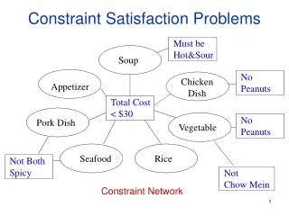
Constraint Satisfaction Problems • What is a CSP? • Finite set of variables X1, X2, …, Xn • Nonempty domain of possible values for each variable D1, D2, …, Dn • Finite set of constraints C1, C2, …, Cm • Each constraint Ci limits the values that variables can take, • e.g., X1 ≠ X2 • Each constraint Ci is a pair <scope, relation> • Scope = Tuple of variables that participate in the constraint. • Relation = List of allowed combinations of variable values. May be an explicit list of allowed combinations. May be an abstract relation allowing membership testing and listing. • CSP benefits • Standard representation pattern • Generic goal and successor functions • Generic heuristics (no domain specific expertise).
CSPs --- what is a solution? • A state is an assignment of values to some or all variables. • An assignment is complete when every variable has a value. • An assignment is partial when some variables have no values. • Consistent assignment • assignment does not violate the constraints • A solution to a CSP is a complete and consistent assignment. • Some CSPs require a solution that maximizes an objective function. • Examples of Applications: • Scheduling the time of observations on the Hubble Space Telescope • Airline schedules • Cryptography • Computer vision -> image interpretation • Scheduling your MS or PhD thesis exam
CSP example: map coloring • Variables: WA, NT, Q, NSW, V, SA, T • Domains: Di={red,green,blue} • Constraints:adjacent regions must have different colors. • E.g. WA NT
CSP example: map coloring • Solutions are assignments satisfying all constraints, e.g. {WA=red,NT=green,Q=red,NSW=green,V=red,SA=blue,T=green}
Graph coloring • More general problem than map coloring • Planar graph = graph in the 2d-plane with no edge crossings • Guthrie’s conjecture (1852) Every planar graph can be colored with 4 colors or less • Proved (using a computer) in 1977 (Appel and Haken)
Constraint graphs • Constraint graph: • nodes are variables • arcs are binary constraints • Graph can be used to simplify search • e.g. Tasmania is an independent subproblem • (will return to graph structure later)
Varieties of CSPs • Discrete variables • Finite domains; size dO(dn) complete assignments. • E.g. Boolean CSPs: Boolean satisfiability (NP-complete). • Infinite domains (integers, strings, etc.) • E.g. job scheduling, variables are start/end days for each job • Need a constraint language e.g StartJob1 +5 ≤ StartJob3. • Infinitely many solutions • Linear constraints: solvable • Nonlinear: no general algorithm • Continuous variables • e.g. building an airline schedule or class schedule. • Linear constraints solvable in polynomial time by LP methods.
Varieties of constraints • Unary constraints involve a single variable. • e.g. SA green • Binary constraints involve pairs of variables. • e.g. SA WA • Higher-order constraints involve 3 or more variables. • Professors A, B,and C cannot be on a committee together • Can always be represented by multiple binary constraints • Preference (soft constraints) • e.g. red is better than green often can be represented by a cost for each variable assignment • combination of optimization with CSPs
CSP as a standard search problem • A CSP can easily be expressed as a standard search problem. • Incremental formulation • Initial State: the empty assignment {} • Actions (3rd ed.), Successor function (2nd ed.): Assign a value to an unassigned variable provided that it does not violate a constraint • Goal test: the current assignment is complete (by construction it is consistent) • Path cost: constant cost for every step (not really relevant) • Can also use complete-state formulation • Local search techniques (Chapter 4) tend to work well
CSP as a standard search problem • Solution is found at depth n (if there are n variables). • Consider using BFS • Branching factor b at the top level is nd • At next level is (n-1)d • …. • end up with n!dn leaves even though there are only dn complete assignments!
Commutativity • CSPs are commutative. • The order of any given set of actions has no effect on the outcome. • Example: choose colors for Australian territories one at a time • [WA=red then NT=green] same as [NT=green then WA=red] • All CSP search algorithms can generate successors by considering assignments for only a single variable at each node in the search tree there are dn leaves (will need to figure out later which variable to assign a value to at each node)
Backtracking search • Similar to Depth-first search, generating children one at a time. • Chooses values for one variable at a time and backtracks when a variable has no legal values left to assign. • Uninformed algorithm • No good general performance
Comparison of CSP algorithms on different problems Median number of consistency checks over 5 runs to solve problem Parentheses -> no solution found USA: 4 coloring n-queens: n = 2 to 50 Zebra: see exercise 6.7 (3rd ed.); exercise 5.13 (2nd ed.)
Improving CSP efficiency • Previous improvements on uninformed search introduce heuristics • For CSPS, general-purpose methods can give large gains in speed, e.g., • Which variable should be assigned next? • In what order should its values be tried? • Can we detect inevitable failure early? • Can we take advantage of problem structure? Note: CSPs are somewhat generic in their formulation, and so the heuristics are more general compared to methods in Chapter 4
Minimum remaining values (MRV) var SELECT-UNASSIGNED-VARIABLE(VARIABLES[csp],assignment,csp) • A.k.a. most constrained variable heuristic • Heuristic Rule: choose variable with the fewest legal moves • e.g., will immediately detect failure if X has no legal values
Degree heuristic for the initial variable • Heuristic Rule: select variable that is involved in the largest number of constraints on other unassigned variables. • Degree heuristic can be useful as a tie breaker. • In what order should a variable’s values be tried?
Least constraining value for value-ordering • Least constraining value heuristic • Heuristic Rule: given a variable choose the least constraining value • leaves the maximum flexibility for subsequent variable assignments
Forward checking • Can we detect inevitable failure early? • And avoid it later? • Forward checking idea: keep track of remaining legal values for unassigned variables. • Terminate search when any variable has no legal values.
Forward checking • Assign {WA=red} • Effects on other variables connected by constraints to WA • NT can no longer be red • SA can no longer be red
Forward checking • Assign {Q=green} • Effects on other variables connected by constraints with WA • NT can no longer be green • NSW can no longer be green • SA can no longer be green • MRV heuristic would automatically select NT or SA next
Forward checking • If V is assigned blue • Effects on other variables connected by constraints with WA • NSW can no longer be blue • SA is empty • FC has detected that partial assignment is inconsistent with the constraints and backtracking can occur.
X1 {1,2,3,4} X2 {1,2,3,4} 1 2 3 4 1 2 3 4 X3 {1,2,3,4} X4 {1,2,3,4} Example: 4-Queens Problem
X1 {1,2,3,4} X2 {1,2,3,4} 1 2 3 4 1 2 3 4 X3 {1,2,3,4} X4 {1,2,3,4} Example: 4-Queens Problem
X1 {1,2,3,4} X2 { , ,3,4} 1 2 3 4 1 2 3 4 X3 { ,2, ,4} X4 { ,2,3, } Example: 4-Queens Problem
X1 {1,2,3,4} X2 { , ,3,4} 1 2 3 4 1 2 3 4 X3 { ,2, ,4} X4 { ,2,3, } Example: 4-Queens Problem
X1 {1,2,3,4} X2 { , ,3,4} 1 2 3 4 1 2 3 4 X3 { , , , } X4 { , ,3, } Example: 4-Queens Problem
X1 {1,2,3,4} X2 { , ,,4} 1 2 3 4 1 2 3 4 X3 { ,2, ,4} X4 { ,2,3, } Example: 4-Queens Problem
X1 {1,2,3,4} X2 { , ,,4} 1 2 3 4 1 2 3 4 X3 { ,2, ,4} X4 { ,2,3, } Example: 4-Queens Problem
X1 {1,2,3,4} X2 { , ,,4} 1 2 3 4 1 2 3 4 X3 { ,2, , } X4 { , ,3, } Example: 4-Queens Problem
X1 {1,2,3,4} X2 { , ,,4} 1 2 3 4 1 2 3 4 X3 { ,2, , } X4 { , ,3, } Example: 4-Queens Problem
X1 {1,2,3,4} X2 { , ,3,4} 1 2 3 4 1 2 3 4 X3 { ,2, , } X4 { , , , } Example: 4-Queens Problem
Comparison of CSP algorithms on different problems Median number of consistency checks over 5 runs to solve problem Parentheses -> no solution found USA: 4 coloring n-queens: n = 2 to 50 Zebra: see exercise 5.13
Constraint propagation • Solving CSPs with combination of heuristics plus forward checking is more efficient than either approach alone • FC checking does not detect all failures. • E.g., NT and SA cannot be blue
Constraint propagation • Techniques like CP and FC are in effect eliminating parts of the search space • Somewhat complementary to search • Constraint propagation goes further than FC by repeatedly enforcing constraints locally • Needs to be faster than actually searching to be effective • Arc-consistency (AC) is a systematic procedure for constraing propagation
Arc consistency • An Arc X Y is consistent if for every value x of X there is some value y consistent with x (note that this is a directed property) • Consider state of search after WA and Q are assigned: SA NSW is consistent if SA=blue and NSW=red
Arc consistency • X Y is consistent if for every value x of X there is some value y consistent with x • NSW SA is consistent if NSW=red and SA=blue NSW=blue and SA=???
Arc consistency • Can enforce arc-consistency: Arc can be made consistent by removing blue from NSW • Continue to propagate constraints…. • Check V NSW • Not consistent for V = red • Remove red from V
Arc consistency • Continue to propagate constraints…. • SA NT is not consistent • and cannot be made consistent • Arc consistency detects failure earlier than FC
Arc consistency checking • Can be run as a preprocessor or after each assignment • Or as preprocessing before search starts • AC must be run repeatedly until no inconsistency remains • Trade-off • Requires some overhead to do, but generally more effective than direct search • In effect it can eliminate large (inconsistent) parts of the state space more effectively than search can • Need a systematic method for arc-checking • If X loses a value, neighbors of X need to be rechecked: i.e. incoming arcs can become inconsistent again (outgoing arcs will stay consistent).
Arc consistency algorithm (AC-3) function AC-3(csp) return the CSP, possibly with reduced domains inputs: csp, a binary csp with variables {X1, X2, …, Xn} local variables: queue, a queue of arcs initially the arcs in csp while queue is not empty do (Xi, Xj) REMOVE-FIRST(queue) if REMOVE-INCONSISTENT-VALUES(Xi, Xj)then for each Xkin NEIGHBORS[Xi] do add (Xi, Xj) to queue function REMOVE-INCONSISTENT-VALUES(Xi, Xj) returntrue iff we remove a value removed false for eachxin DOMAIN[Xi] do if no value y inDOMAIN[Xj]allows (x,y) to satisfy the constraints between Xi and Xj then delete x from DOMAIN[Xi]; removed true return removed (from Mackworth, 1977)
Complexity of AC-3 • A binary CSP has at most n2 arcs • Each arc can be inserted in the queue d times (worst case) • (X, Y): only d values of X to delete • Consistency of an arc can be checked in O(d2) time • Complexity is O(n2 d3) • Although substantially more expensive than Forward Checking, Arc Consistency is usually worthwhile.
K-consistency • Arc consistency does not detect all inconsistencies: • Partial assignment {WA=red, NSW=red} is inconsistent. • Stronger forms of propagation can be defined using the notion of k-consistency. • A CSP is k-consistent if for any set of k-1 variables and for any consistent assignment to those variables, a consistent value can always be assigned to any kth variable. • E.g. 1-consistency = node-consistency • E.g. 2-consistency = arc-consistency • E.g. 3-consistency = path-consistency • Strongly k-consistent: • k-consistent for all values {k, k-1, …2, 1}