Linear Programming
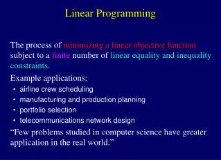
Linear Programming. Introduction. What is Linear Programming?. A Linear Programming model seeks to maximize or minimize a linear function , subject to a set of linear constraints . What are linear functions?. Linear function in 2 variables. No X 1 2 , X 1 /X 2 , e -X2 , X 1 , etc.

Linear Programming
E N D
Presentation Transcript
Linear Programming Introduction
What is Linear Programming? • A Linear Programming model seeks to maximize or minimize a linear function, subject to a set of linear constraints.
What are linear functions? Linear function in 2 variables No X12, X1/X2, e-X2,X1, etc. • y = mx+b is the equation of a straight line • e.g. y = -4/3 x +6 • Multiplying by 3 and rearranging: 4x + 3y = 18 Alinear function consists of the sum of positive, negative or 0 constants times variables; e.g. 5X1 - 4X2 + 0X3 + 6X4 is a linear function in 4 variables.
What are Linear Constraints? • Linear constraints have the form: <Linear Function><has some relation to><a constant> • The relation is one of the following: , = , ---- they all contain the “equal to” part Examples: 4X1 + 5X2 - 6X3 + 2X534 2X1 - 5X2 + 1X447 - 2X2 + 8X3 + 9X4 + 2X5=67 X1 0 X5 0
Example of a Linear Program Subject to X1 0, X2 0, X3 0, X4 0 MAX 4X1 + 7X3 - 6X4 s.t. 2X1 + 3X2 - 2X4 = 20 - 2X2 + 9X3 + 7X4 10 -2X1 + 3X2 + 4X3 + 8X4 35 X2 5 All X’s 0
Another Example MIN 6X1 + 8X2 + 11X3 + 10X4 + 5X5 + 14X6 S.T. X1 + X2 + X3 20 X4 + X5 + X6 30 X1 + X4 = 12 X2 + X5 = 15 X3 + X6 = 22 All X’s 0
Components of a Linear Programming Model • A linear programming model consists of: • A set of decision variables • A (linear) objective function • A set of (linear) constraints
Why are Linear Programs Important? • Many real world problems lend themselves to linear programming modeling. • Other real world problems can be approximated by linear models. • There are well-known successful applications in: • Manufacturing, Marketing, Finance (investment), Advertising, Agriculture, Energy, etc. • There are efficient solution techniques and software programs that solve linear programming models. • The output generated from linear programming packages provides useful “what if” analysis.
Linear Programming Assumptions • The parameter values are known with certainty. • The objective function and constraints exhibit constant returns to scale. • There areno interactionsbetween the decision variables (additivity assumption). • Continuityof the decision variables means they can take on any value within a given feasible range. • Integer programming models can only take on integer values within a given feasible range.
Example • Galaxy Industries manufactures two toy gun models: • Space Rays: Each dozen nets an $8 profit and • Requires 2 lbs. of plastic; 3 minutes of production time • Zappers: Each dozen nets a $5 profit and • Requires 1 lb. of plastic; 4 minutes of production time • Weekly resource limits • 1000 pounds of plastic; 40 hours of production time • Weekly production limits • Maximum 700 dozen total units • Space Rays cannot exceed Zappers by more than 350 dozen
Current Production • Current reasoning calls for a production plan that: • Produces as much as possible of the more profitable product, Space Ray ($8 profit per dozen). • Uses any left over resources to produce Zappers ($5 profit per dozen), while remaining within the marketing guidelines of 700 total dozen produced and Space Rays – Zappers ≤ 350. • Using a simple spreadsheet, letting the (cell for production of Zappers) = (cell for production of Space Rays – 350), trial and error gives the following good solution that uses all the available weekly plastic: Space Rays = 450 dozen; Zappers = 100 dozen; Profit = 8(450) + 5(100) = $4100 This is a good solution – Can we do better?
The Mathematical Model • Recall a mathematical model consists of: • Set of decision variables • Objective function • Constraints • Decision Variables (Include both a measurement unit (dozens) and a time unit (week)) X1 = dozens of Space Rays produced weekly X2 = dozens of Zappers produced weekly
2. OBJECTIVE FUNCTION • Objective is to maximize the total weekly profit. How much profit will be made each week? • How much profit will • be made weekly from • Space Rays? • How much profit will • be made weekly from • Zappers? $5 per dozen $8 per dozen Make X2 dozen Zappers per week Make X1 dozen Space Rays per week 5X2 8X1 + MAX 8X1 + 5X2
3. Constraints -- PLASTIC • At most 1000 pounds of plastic available weekly. How much will be used? • How much plastic will • be used weekly making • Space Rays? • How much plastic will • be used weekly making • Zappers? 1 lb per dozen 2 lbs per dozen Make X2 dozen Zappers per week Make X1 dozen Space Rays per week 1X2 2X1 + 2X1 + 1X2 1000
Constraints -- Production Time • At most 40 hours = 40x60 = 2400 minutes available weekly. How much will be used? • How many minutes will • be used weekly making • Space Rays? • How many minutes will • be used weekly making • Zappers? 4 min per dozen 3 min per dozen Make X2 dozen Zappers per week Make X1 dozen Space Rays per week 4X2 3X1 + 3X1 + 4X2 2400
Constraints -- Max Production • At most 700 dozen total units can be produced weekly. How many will be produced? • How many dozen • Space Rays are • produced weekly? • How many dozen • Zappers are • Produced weekly? Make X1 dozen Space Rays per week Make X2 dozen Zappers per week X1 + X2 X1 + X2 700
Constraints -- Product Mix Amount (in dozens) Space Rays exceed Zappers • Space Rays can be at most 350 dozen units greater than Zappers each week. How many more dozen units of Space Rays will be produced weekly? • How many dozen • Space Rays are • produced weekly? • How many dozen • Zappers are • Produced weekly? Make X2 dozen Zappers per week Make X1 dozen Space Rays per week X2 - X1 X1 - X2 350
Constraints -- Nonnegativity • Cannot produce a negative amount of Space Rays or Zappers X1 0 X2 0 or All X’s 0
The Complete Galaxy IndustriesLinear Programming Model MAX 8X1 + 5X2 s.t. 2X1 + 1X2≤ 1000 (Plastic) 3X1 + 4X2 ≤ 2400 (Prod. Time) X1 + X2 ≤ 700 (Total Prod.) X1 - X2 ≤ 350 (Mix) All X’s ≥ 0
Review • A linear program seeks to maximize or minimize a linear objective subject to linear constraints. • Many problems are or can be approximated by linear programming models. • Linear programs possess the features of: • Certainty, Constant Returns to Scale, Additivity and Continuity • There exists efficient algorithms for solving linear programs that provide many sensitivity analyses as a by-product.

