Download
1 / 15
190 likes | 670 Vues
Motions and Mooring Lines of Floaters. Lecture in TMR 4195, March 20, 2007 Sverre Haver. Floater, mooring lines and risers. z. Wind. x(t). Waves. x. Current. f(t). Risers. Mooring Lines. Anchors. Force processes. Wind (mean force and slowly varying force) Current (mean force)

E N D
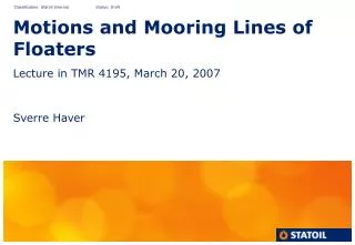
Motions and Mooring Lines of Floaters Lecture in TMR 4195, March 20, 2007 Sverre Haver
Floater, mooring lines and risers z Wind x(t) Waves x Current f(t) Risers Mooring Lines Anchors
Force processes • Wind (mean force and slowly varying force) • Current (mean force) • Waves ( wave frequent force, mean slow drift force, slowly varying force)Cold regions: • Ice force (mean force and moderate impact forces)In case of possibility of collicion with ice bergs,moorings and risers are disconnected and position is left.
Problems to be considered • Extreme offset to ensure that risers are not put at risk; characteristic value q-probability offset or mean offset of q-probability sea state. Check with actual rules and regulations. • Mooring line loads; characteristic value is expected largest load in q-probability sea state (q=10-2 typically). • Line loads acting on anchors and hull; characteristic loads are q-probability loads for anchor (typically) and mooring line breaking load for hull (to ensure that mooring line fails before tearing hull open)
Offset, x(t), and mooring line load, f(t), components • Mean offset, mean line load, forcinge processes:mean wind force, mean wave drift force, current force, ice force • Wave frequency offset and line load, forcing process:Surface waves, typical period band 5-25s. • Low frequency force, forcing processes:Turbulent wind, slowly varying wave drift force.Typical period band: natural periods in surge, sway and yaw, and, occasionally, natural periods in pitch and roll (if it is exceeding say 30-40s)
Static or dynamic analysis • Ice response and current: Quasi-static analysis, typically. • Wind and waves: Dynamic analysis with respect to offset both for line loads and offset.Line behaviour: Often a quasi-static line behaviour is assumed, i.e.line dynamics are neglected. NB! Safety factor requirements for line loads depend on whether a quasistatic or dynamic line behaviour is accounted for. Intact case: 3.0 for quasistatic analysis 2.5 for dynamic analysis
Linear or Non-linear Analysis • A linearized analysis is often performed, i.e. stiffness and damping are linearized around proper offset values. (MIMOSA is a computer program utilizing a linearized analysis.)* Slow drift analysis: Linearization is made around mean static + mean slow frequency offset.* Wave drift analysis: Linearization is made aroun mean static offset+ extreme slow drift offset. • A coupled non-linear analysis can be done by solving the equations of motions in the time domain, e.g floater motion by SIMO and corresponding mooring line motion by Riflex.
Steps involved in linearized analysis1: Mean values due to mean wind, vw, and mean current, vc. • Loads are found by multiplying vw**2 and vc**2 with proper load coefficients for various directions and drafts. • These coefficients are most accurately determined by wind tunnel tests. • The mean load or offset is here denoted by
2. Wave frequency values • Wave frequency results found from frequency domain analyses, i.e.: • Expected maximum during a 3-hour period: Wave spectrum Response spectrum Linearized transfer function sR = response st.dev. = no of WF cycles in3 hours
3. Low frequency response3.1 Wind induced • Wind induced response is estimated using wind spectrum and a linearized mechanical system. Wind induced force: Mean load,accounted for above Varying wind force, vw,turb isGaussian, i.e. the variable forceis Gaussian (frequency domainsolution is convenient) Expected 3-hour maximum reads:
3.2 Wave induced low frequency motion • More complicated, we will not og into detail. • Force, is proportinal to , i.e. force is non-Gaussian.Force maxima follow an exponential distribution. (Show why?)(Assume that maxima of the wave process follow a Rayleigh model and use transformation of variables.) • Low frequency motion very much effected by resonance. This tends to”Gaussinize” the response. Response process between a Gaussian process and a squared Gaussian process and response maxima follow a model between a Rayleigh model and an expential model. Denote here 3-hour maximaby:
3 Low frequency response • Resulting low frequency resoponse: In this formula it is assumed that wind induced and wave inducedlow frequency 3-hour extremes are independent.
4 Resulting extreme response • Resulting extreme response is a challenging theoretical results. Hereit is approximated by the following formula (empirical results shown to give reasonable results): Significant response amplitude is equal to two times the standard deviation of the corresponding response component. More accurate results requires solving the equation of motion in time domain or a large number of 3-hour model tests.
Model testing • For very complex problems, it may not be possible to identify the short term probabilistic structure of the target response quantity. For such model testing is a good alternative. • Prior to the execution of the model test program, one should spend some time on a careful consideration of what is the aim of the model test:a) Is the model test performed primarily for calibrating computer programs for time domain or frequency domain considerations?b) Or, is the model test results meant to be used for obtaining characteristic response?
Test type b) • Use the environmental contour line principle for selecting sea states. 10**(-2) contours if 10**(-2) responses are requested, 10**(-4) contours if 10**(-4) responses are requested. • Select a number (4-6) of different sea states enveloping the range on the contours expected to represent the worst sea states. • Perform some few 3-hour (full scale time) tests for the selected sea states. The number of tests can be 4-6 of each sea states. • Select which sea state that is the worst sea state in view of target response quantity and execute a number of additional realizations for this sea state. • Identify the 3-hour extremes for this sea state and fit a proper probabilistic model to these observed extremes. • Estimate the q-proability response by the 90% (85 – 95)% percentile value of this distribution.