
SlideServe
Menu
Préférences
© SlideServe · v2026

Feedback System Stability

yoshio-maldonado avatar
6 diapositives · 590 Views · Nov 01, 2014

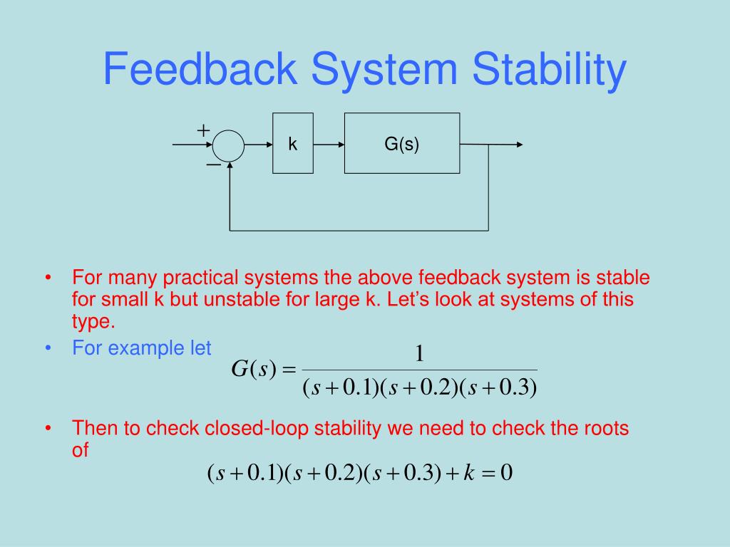
k. G(s). Feedback System Stability. For many practical systems the above feedback system is stable for small k but unstable for large k. Let’s look at systems of this type. For example let Then to check closed-loop stability we need to check the roots of. Closed-loop Poles. Let Then
Feedback System Stability - slide 1
01 / 6Feedback System Stability
1 / 17

Télécharger la présentation

Feedback System Stability
Une image / un lien ci-dessous est fourni (tel quel) pour télécharger la présentation

Politique de téléchargement : le contenu du site vous est fourni TEL QUEL pour votre information et votre usage personnel ; il ne peut être vendu, concédé sous licence ni partagé sur d’autres sites sans l’accord de son auteur.Le contenu vous est fourni TEL QUEL, pour votre information et votre usage personnel uniquement. Téléchargez la présentation en cliquant sur ce lien. Lors du téléchargement, si vous ne parvenez pas à télécharger une présentation, l’éditeur a peut-être supprimé le fichier de son serveur.Pendant le téléchargement, si vous ne parvenez pas à obtenir une présentation, le fichier a peut-être été supprimé par l’éditeur.

F I N

Plus de contenu associé

Transcription de la présentation
  1. k G(s) Feedback System Stability • For many practical systems the above feedback system is stable for small k but unstable for large k. Let’s look at systems of this type. • For example let • Then to check closed-loop stability we need to check the roots of

  2. Closed-loop Poles • Let • Then • The sum of closed-loop poles is constant and equal to -0.6.

  3. Closed-loop poles and k • As k is increased from 0 to 0.05, the closed-loop system has only one real and two imaginary poles. • The real pole goes more negative as k increases so the real part of the imaginary poles must become less negative since the sum of the poles is constant. • This means as k increases the real part of the closed-loop imaginary poles will become positive. • And so there will be one value of k, let’s call it k*, for which the real part of the imaginary closed-loop poles will be zero, i.e, 2 , 3 is ±j* for some *.

  4. Is k < k* or k=k* or k > k*? • Find out k* from the frequency response and if our k is less than k* the closed-loop system is stable, if k is equal to k* it’s marginally stable and if k is greater than k* then it’s unstable.

  5. //cubic polynomial roots //2 August 2005 //exec('cubic.sce') s=poly(0,'s'); k=0.05;//0.06; x=[-0.8:0.01:0.0]; x1=0.1;x2=0.2;x3=0.3; y=(x+x1).*(x+x2).*(x+x3)+k; f1=scf(1);clf(f1,'reset'); plot2d(x,y);xgrid; xtitle('Third Order Polynomial', 'x','y'); den=poly([x1*x2*x3+k (x1*x2+x1*x3+x2*x3) (x1+x2+x3) 1],"x","coeff"); abc=roots(den) s1=sum(abc); //sum of the three roots disp(s1, 'sum of roots = ') //s1=sum(abc) //sum of the three roots h=syslin('c',1,x1*x2*x3+(x1*x2+x1*x3+x2*x3)*%s+(x1+x2+x3)*%s^2+%s^3); [g,fr]=g_margin(h); f2=scf(2);//clf(f2,'reset'); bode(h,0.001,10);