Download
1 / 1
20 likes | 163 Vues
Land Cover Class. Forest Inventory. Landsat Map. Forest. 5.478. 4.755. Bog. 0.725. 0.695 1. Water. 0.217 2. 0.123 1. Shrubland/grassland. 0.461. 0.213 1,3. Land Cover and Forest Biomass in the St. Petersburg Region of Russia: Integrating Landsat with Forest Inventory Data

E N D
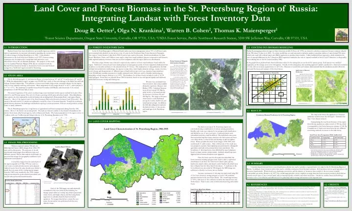
Land Cover Class Forest Inventory Landsat Map Forest 5.478 4.755 Bog 0.725 0.695 1 Water 0.217 2 0.123 1 Shrubland/grassland 0.461 0.213 1,3 Land Cover and Forest Biomass in the St. Petersburg Region of Russia: Integrating Landsat with Forest Inventory Data Doug R. Oetter1, Olga N. Krankina1, Warren B. Cohen2, Thomas K. Maiersperger1 1Forest Science Department, Oregon State University, Corvallis, OR 97331, USA; 2USDA Forest Service, Pacific Northwest Research Station, 3200 SW Jefferson Way, Corvallis, OR 97331, USA INTRODUCTION Russian forests have been identified as a potentially important sink for carbon sequestration, but accurate information regarding the current status of carbon storage is lacking (Krankina et al. 1996). Using detailed information at the local forest level (Kukuev et al. 1997), remote sensing techniques may be employed to extrapolate land and forest cover information across the vast Russian landscape. The purpose of this study is to use Landsat Thematic Mapper (TM) data in conjunction with the Russian Forest Inventory System to characterize forest cover and biomass storage for a 76,850 km2 region around St. Petersburg. 1.1 INTRODUCTION 2.3 FOREST INVENTORY DATA In the St. Petersburg region of Russia all lands under state forest management (about 75% of all forest lands) are inventoried with detailed on-site surveys every 10 years by the Northwest State Forest Inventory Enterprise. Two types of forest inventory data from 1992-93 survey were used in this study. Stand–level databases for three forests (Roschino, Tosno, and Volkhov) were used to map forest stand attributes (species composition and biomass), while regional summary inventory data was used for comparison with the region land-cover classification. The three ranger districts were selected to represent the variation in forest stand attributes found within the region. Field crews surveyed each forest stand polygon (a homogeneous patch of forest vegetation) delineated from air photos on the entire territory of the selected forests (97,714 ha). The standard set of data gathered in the field included site productivity and drainage, tree species composition, mean height, diameter and age, canopy structure, wood volume, and characteristics of different types of land without tree cover (e.g., clearcuts, bogs, meadows). Over 200 different variables measured or visually estimated in the field were used to describe stand polygons, depending on land category (Kukuev et al. 1997). The databases for all three forests included a total of 12,791 stand polygons. From these we selected about 1500 for analysis, based on size and spectral signals, and randomly subdivided them into testing and training sets. Rather than mapping carbon storage via forest structure models (Cohen et al. 1996), we elected to calculate continuous biomass estimates directly from TM values (Cohen et al. 2001). To reduce model bias, we used canonical correlation analysis to produce indices of transformed TM values which were used with reduced major axis (RMA) regression to produce linear models. Unlike traditional linear regression, which minimizes the sum of squared differences in the Y direction, RMA regression minimizes the sum of squared residuals in both X and Y directions (orthogonally), thus reducing bias of the fit (Curran and Hay 1986). In the graph below, predicted and observed biomass values for the testing data set are shown by species group. Each species was modeled separately, yet the average error is low throughout. Overall, for the testing data, this modeling approach yielded a predicted vs. observed correlation of 0.62, with a root mean squared error of 43.5 t/ha. Measures of model bias and variance demonstrated that the prediction models effectively recreated the mean and variance of the observations. 2.5 CONTINUOUS BIOMASS MODELING Forest Inventory Polygons And Landsat Imagery The Tosno forest polygons are projected in the image to the right over the core Landsat scene (bands 7, 5, 3 displayed as red, green, blue). This shows the polygon boundaries as they were digitized, with the entire forest classified into over 20 different land cover classes for 2572 polygons. In the blow-up image below, the original vector polygons have been buffered inward by 50 m and reselected for a minimum area of 2 ha. This procedure allowed us to reduce the number of polygons containing landscape boundaries, thus improving the homogeneous signal of the polygon for statistical analysis. Application of Biomass Predictions Applying the biomass model predictions to the source data creates a continuous spatial image, with pixel values in average biomass (t/ha) over each pixel. This image has been truncated so that negative values have been recoded to 1. The enlargement below details the area within the box at the right. 2.1 STUDY AREA STUDY AREA The St. Petersburg region of northwestern Russia is located between 58° and 62° N and between 28° and 36° E. While the administrative region occupies over 100,000 km2, much of that area belongs to the Baltic Sea and Lake Ladoga, Europe’s largest lake. The influence of these water bodies helps create a maritime climate for the region, with cool wet summers and long cold winters. Mean temperature in July ranges from16° to 18° C, and in January it is -7° to -11° C. The landscape is typically frozen from November until March, such that much of the annual precipitation of 600-800 mm falls as snow. The natural vegetation of the area is southern taiga; major dominant conifer species include Scots pine (Pinus sylvestris L.) and Norway spruce (Picea abies (L.) Karst.), growing in both pure and mixed stands. After disturbance, these species are often replaced by northern hardwoods, including birch (Betula pendula Roth.) and aspen (Populus tremula L.). Most of the region is part of the East-European Plain with elevations between 0 and 250 m amsl. The terrain is flat and consists of ancient sea sediments covered by a layer of moraine deposits. Toward the northwest, glacial features dominate the landscape and bedrock topology is more prominent. Soils are mostly podzols on deep loamy to sandy sediments. The St. Petersburg region has a long history of agricultural and forest management dating from the 18th century. Most of the forests are second-growth. The land-use history is similar to that found in Scandinavia but distinct from many other boreal regions, such as Siberia and Alaska. The human population of the region is close to 7 million, with over 5 million people living in the city of St. Petersburg (Krankina et al. 1998). r = 0.62 RMSE = 43.5 t/ha Biomass was calculated from forest inventory data using available allometric equations (Alexeyev and Birdsey 1998). Calculated biomass stores do not exceed 310 Mg/ha while in 64% of all stand records the biomass is between 100 and 200 Mg/ha. The range of biomass observations is well distributed among the conifer, hardwood, and mixed species groups. In addition, the field data adequately represent the limited variety of tree species and stand ages in St. Petersburg region. 3.1 RESULTS The map at left shows the application of biomass prediction models across the full region. Estimates less than 1 have been truncated. Extrapolating the total forest biomass of the region from the raw predictions yields a result of 585 Tg, which is comparable to the Forest Inventory estimate of 506 Tg. Comparisons of land cover areas from the two different accounting methods are shown in the table below. Continuous Biomass Predictions for St. Petersburg Region 2.4 LAND COVER MAPPING The land cover map of St. Petersburg region was constructed using a combination of remote sensing procedures. Initially, each scene was subjected to an unsupervised classification and labeled as one of ten cover types. Confused clusters were reclassified until they could be defined. The individual scenes were then mosaicked together using a decision rule that conserved forest over other classes, so that clouds and clearings would not replace forest. Where possible the more recent images (1994-1995) were used instead of earlier scenes. After a full mosaic of the study area was prepared, extensive hand digitizing was performed to distinguish agriculture and built environments from forest and shrub. The boundaries of developed areas were delimited by expert judgment based on shape, texture, and proximity. Similarly, mined bogs were digitized where human alterations were apparent. Once the forest area for the region was identified, the forest inventory training polygons were used to drive a supervised classification to produce five forest cover classes (pine, spruce, hardwood, mixed conifer, and mixed conifer/hardwood), which were later collapsed into the three final forest classes. A small area in the far northwest was uncovered by TM imagery; the MSS image was sufficient to classify it as forest, but not further. Accuracy assessment of this map was performed using 822 of the forest inventory testing polygons as well as 300 randomly generated points in the non-forest classes. The overall map accuracy is 70.9%, with most of the confusion found in the mixed forest and shrub classes. There is also some confusion between bog and conifer forest. Land Cover Characterization of St. Petersburg Region, 1986-1995 Land Cover Area Comparison Table (million ha) Thirteen separate Landsat TM and one Multi-Spectral Sensor (MSS) images from 1986-1995 were used in this project. The presence of clouds necessitated using images from different years and different seasons. Before data analysis could begin, we processed the images for geographic rectification and radiometric normalization. A cloud free image from the central part of the region acquired on 19 May 1992 was used as a ‘core’ scene to which all other scenes were adjusted. Adjacent scenes from the same decade were shifted to match the core scene in the overlap region; images from the 1980’s were matched to the 1990’s images using an automated tie-point selection procedure and second-order polynomial transformation. 2.2 IMAGE PRE-PROCESSING Landsat Band 4 Mosaic 1 Areas for these land-cover classes are available only for lands under state forest management or about 75% of all ‘Forest Fund Lands’ 2 Inland only; excluding the Baltic Sea and Lake Ladoga 3 Included in this category are open plantations, clearcuts, transmission and survey lines, roads, hay lots, and wastelands A Landsat-based land and forest cover classification scheme was used to produce a regional land cover map for the St. Petersburg Region of Russia. In addition, forest inventory plots were used to calculate continuous forest biomass estimates. Both products were in good agreement with inventory-based results. While cloud cover, landscape conversion, and the absence of inventory data outside of the core scene certainly confounded our results (Homer et al. 1997), the overall maps provide a more complete coverage than the forest inventory method, which did not include several types of tree-covered lands, such as municipal parks, orchards, and other treed areas. Overall the satellite-based methodology promises to be a cost-effective and efficient tool for gathering carbon storage information at the regional scale. 3.2 SUMMARY Training forest location Study area boundary 4.1 REFERENCES Alexeyev, V. A. and R. A. Birdsey. 1998. Carbon storage in forests and peatlands of Russia. USDA Forest Service General Technical Report NE-244. Cohen, W. B., M. E. Harmon, D. O. Wallin, and M. Fiorella. 1996. Two decades of carbon flux from forests of the Pacific Northwest. BioScience 46(11):836-844. Cohen, W. B., T. K. Maiersperger, T. A. Spies, and D. R. Oetter. 2001. Modelling forest cover attributes as continuous variables in a regional context with Thematic Mapper data. International Journal of Remote Sensing (in press). Curran, P. J., and A. M. Hay. 1986. The importance of measurement error for certain procedures in remote sensing at optical wavelengths. Photogrammetric Engineering & Remote Sensing 52(2):229-241. Homer, C. G., R. D. Ramsey, T. C. Edwards, Jr., and A. Falconer. 1997. Landscape cover-type modeling using a multi-scene Thematic Mapper mosaic. Photogrammetric Engineering & Remote Sensing 63(1):59-67. Krankina, O. N., M. Fiorella, W. Cohen, and R. F. Treyfeld. 1998. The use of Russian forest inventory data for carbon budgeting and for developing carbon offset strategies. World Resource Review 10(1):52-66. Krankina, O. N., M. E. Harmon, and J. K. Winjum. 1996. Carbon storage and sequestration in the Russian forest sector. Ambio 25(4):284-288. Kukuev, Y.A., O. N. Krankina and M. E. Harmon. 1997. The forest inventory system in Russia. Journal of Forestry 95(9):15-20. 4.2 CREDITS This project is funded by the NASA Land Cover – Land Use Change Program (LCLUC). The authors gratefully acknowledge the significant efforts of Rudolf Treyfeld of the NW Forest Inventory Enterprise, St. Petersburg, Russia. For more information, please refer to our web page: http://www.fsl.orst.edu/larse/russia/ Each of the TM images was radiometrically normalized to the core scene by first selecting ‘no-change’ pixels within an overlap area which represented water, forest, and bright objects, and then using linear regression to calculate band-by-band correction equations. For images that did not contact the core scene, the procedure was performed with the next adjacent image. Land Cover Map Error Matrix CORE SCENE