The Normal Distribution

1. The Normal Distribution 15.4 • Understand the basic properties of the normal curve. • Relate the area under a normal curve to z-scores. • Make conversions between raw scores and z-scores. • Use the normal distribution to solve applied problems.

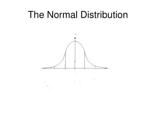
2. The Normal Distribution The normal distribution describes many real-life data sets. The histogram shown gives an idea of the shape of a normal distribution.

3. The Normal Distribution The normal distribution describes many real-life data sets. The histogram shown gives an idea of the shape of a normal distribution. • Examples of Normal Distributions: • Sat Scores • Heights of People • Number of miles before the tires on a car wear out

4. The Normal Distribution

5. The Normal Distribution We represent the mean by μ and the standard deviation by σ. Mu & lower case sigma instead of and s because we are dealing with the whole population.

6. The Normal Distribution • Example: Suppose that the distribution of scores of 1,000 students who take a standardized intelligence test is a normal distribution. If the distribution’s mean is 450 and its standard deviation is 25, a) how many scores do we expect to fall between 425 and 475? b) how many scores do we expect to fall above 500? (continued on next slide)

7. The Normal Distribution • Solution (a): 425 and 475 are each 1 standard deviation from the mean. Approximately 68% of the scores lie within 1 standard deviation of the mean. • We expect about • 0.68 × 1,000 = 680 scores are in the range 425 to 475. (continued on next slide)

8. The Normal Distribution Solution (b): We know 5% of the scores lie more than 2 standard deviations above or below the mean, so we expect to have 0.05 ÷ 2 = 0.025 of the scores to be above 500. Multiplying by 1,000, we can expect that 0.025 * 1,000 = 25 scores to be above 500.

9. The Normal Distribution • Example: Suppose a distribution has a mean of 10 and a standard deviation of 2. Find the percentage of values between; a) 10 and 12? b) Below 8? (continued on next slide)

10. The Normal Distribution • Example: Suppose a distribution has a man of 10 and a standard deviation of 2. Find the percentage of values between; a) 10 and 12? b) Below 8? (continued on next slide)

11. z-Scores The standard normal distribution has a mean of 0 and a standard deviation of 1. There are tables (see next slide) that give the area under this curve between the mean and a number called a z-score. A z-scorerepresents the number of standard deviations a data value is from the mean. For example, for a normal distribution with mean 450 and standard deviation 25, the value 500 is 2 standard deviations above the mean; that is, the value 500 corresponds to a z-score of 2.

12. z-Scores The next three slides show a table that gives the area under the standard normal curve between the mean and a z-score.

16. z-Scores • Example:Use a table to find the percentage of the data (area under the curve) that lie in the following regions for a standard normal distribution: a) between z= 0 and z= 1.3 b) between z= 1.5 and z= 2.1 c) between z= 0 and z= –1.83 (continued on next slide)

17. z-Scores • Solution (a): The area under the curve between z= 0 and z= 1.3 is shown. Using a table we find this area for the z-score 1.30. We find that A is 0.403 when z= 1.30. We expect 40.3%, of the data to fall between 0 and 1.3 standard deviations above the mean. (continued on next slide)

18. z-Scores • Solution (b): The area under the curve between z= 1.5 and z= 2.1 is shown. We first find the area from z= 0 to z= 2.1 and then subtract the area from z= 0 to z= 1.5. Using a table we get A = 0.482 when z= 2.1, and A = 0.433 when z= 1.5. The area is 0.482 – 0.433 = 0.049 or 4.9% (continued on next slide)

19. z-Scores • Solution (c): Due to the symmetry of the normal distribution, the area between z= 0 and z= –1.83 is the same as the area between z= 0 and z= 1.83. Using a table, we see that A= 0.466 when z= 1.83. Therefore, 46.6% of the data values lie between 0 and –1.83.

20. Converting Raw Scores toz-Scores

21. Converting Raw Scores toz-Scores • Example:Suppose the mean of a normal distribution is 20 and its standard deviation is 3. a) Find the z-score corresponding to the raw score 25. b) Find the z-score corresponding to the raw score 16. (continued on next slide)

22. Converting Raw Scores toz-Scores • Solution (a): We have • We compute (continued on next slide)

23. Converting Raw Scores toz-Scores • Solution (b): We have • We compute

24. Applications • Example:Suppose you take a standardized test. Assume that the distribution of scores is normal and you received a score of 72 on the test, which had a mean of 65 and a standard deviation of 4. What percentage of those who took this test had a score below yours? (continued on next slide)

25. Applications • Example:Suppose you take a standardized test. Assume that the distribution of scores is normal and you received a score of 72 on the test, which had a mean of 65 and a standard deviation of 4. What percentage of those who took this test had a score below yours? • Solution: We first find the z-score that corresponds to 72. (continued on next slide)

26. Applications Using a table, we have that A = 0.460 when z = 1.75. The normal curve is symmetric, so another 50% of the scores fall below the mean. So, there are 50% + 46% = 96% of the scores below 72. (continued on next slide)

27. Applications • Example:Consider the following information: • 1911: Ty Cobb hit .420. Mean average was .266 • with standard deviation .0371. • 1941: Ted Williams hit .406. Mean average was • .267 with standard deviation .0326. • 1980: George Brett hit .390. Mean average was • .261 with standard deviation .0317. • Assuming normal distributions, use z-scores to determine which of the three batters was ranked the highest in relationship to his contemporaries. (continued on next slide)

28. Applications • Solution: • Ty Cobb’s average of .420 corresponded to a z-score of • Ted Williams’s average of .406 corresponded to a z-score of • George Brett’s average of .390 corresponded to a z-score of • Compared with his contemporaries, Ted Williams ranks as the best hitter.

29. Applications • Example: A manufacturer plans to offer a warranty on an electronic device. Quality control engineers found that the device has a mean time to failure of 3,000 hours with a standard deviation of 500 hours. Assume that the typical purchaser will use the device for 4 hours per day. If the manufacturer does not want more than 5% to be returned as defective within the warranty period, how long should the warranty period be to guarantee this? (continued on next slide)