Understanding Random Variables and Their Distributions: Concepts and Examples
This overview explores the concept of random variables (r.v.) in probability theory. It defines random variables as functions that map outcomes from a sample space into real numbers, with examples including coin flips and dice rolls. It distinguishes between discrete and continuous random variables and illustrates their properties, such as the cumulative distribution function (CDF) and density functions. Special distributions like the Gaussian random variable are also discussed, along with methodologies for computing probabilities and evaluating distribution functions.

Understanding Random Variables and Their Distributions: Concepts and Examples
E N D
Presentation Transcript
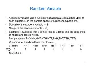
2.1 Random Variable Concept • Given an experiment defined by a sample space S with elements s, we assign a real numberto every saccording to some rule as follows; • X : a function that maps all elements of the sample space into points on the real line
Example 2.1-1 • Rolling a die and flipping a coin • Sample space {H,T} x {1,2, ..., 6} • Let the r.v. be a function X as follows • A coin head (H) outcome -> positive value shown up on the die • A coin tail (T) outcome -> negative and twice value shown up on the die
Example 2.1-2 • The pointer on a wheel of chance is spun • The possible outcomes are the numbers from 0 to 12 marked on the wheel • Sample space {0 < s 12} • Define a r.v. by the function • Points in S map onto the real line as the set {0 < x 144}
2.1 Random Variable Concept • Conditions for a Function to be a Random Variable • Every point in S must correspond to only one value of the r.v. • The set { X x} shall be an event for any real number x • The set {X(s) x} corresponds to those points s in the sample space for which the X(s) does not exceed the number x This means that the set is not a set of numbers but a set of experimental outcomes • The probabilities of the events {X=} and {X=- } shall be 0: • This condition does not prevent X from being either - or for some values of s; it only requires that the prob. of the set of those s be zero The function that maps outcomes in the following manner can not be a r.v. ... ... - -2 -1 0 1 2
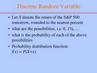
2.1 Random Variable Concept • Discrete and Continuous Random Variables • Discrete r.v.:Having only discrete values • Example 2.1-1 : discrete r.v. defined on a discrete sample space • Continuous r.v. : Having a continuous range of values • Example 2.1-2 : continuous r.v. defined on a continuous sample space • Mixed r.v. : Some of its values are discrete and some are continuous
2.2 Distribution Function • Cumulative Probability Distribution Function – CDF • The probability of the event {X x} : • Depend on x • A function of x • Distribution function of X • Properties ; consider a discrete distribution
2.2 Distribution Function • Discrete Random Variable • If X is a discrete r.v., : stair-step form • Amplitude of a step : probability of occurrence of the value of X where the step occurs • If the values of X are denoted xi, we may write where u(·) is the unit-step function • Using
2.2 Distribution Function Fx(3)=Fx(3+)=1 by the property (6)
Example 2.2-1 • Let X have the discrete values in the set {-1, -0.5, 0.7, 1.5, 3} • The corresponding probabilities {0.1, 0.2, 0.1, 0.4, 0.2}
Example 2.2-2 • Wheel-of-chance experiment
2.3 Density Function • Probability Density Function (PDF) of r.v. X • Existence • If the derivative of FX(x) exists, thenfX(x) exists • If there may be places where dFX(x)/dx is not defined (abrupt change in slope), FX(x) is a function with step-type discontinuities such as in ex. 2.2-2.
2.3 Density Function • Discrete r.v. • Stair-step form distribution function • Description of the derivative of FX(x) at stairsteppoints • Unit-impulse function, (t), used
2.3 Density Function • Unit-Impulse Function (t) • Definition by its integral property • (x) : any continuous function at the point x = x0 • (t) • Can be integrated as a “function” with infinite amplitude, area of unity, and zero duration • The relationship of unit-impulse and unit-step functions • The general impulse function • Shown symbolically as a vertical arrow occurring at the point x=x0 and having an amplitude equal to the amplitude of the step function for which it is the derivative
2.3 Density Function • A discrete r.v. • The density function for a discrete r.v. exists • Using impulse functions to describe the derivative of FX(x) at its stair step points
2.3 Density Function • Properties of Density Functions
Example 2.3-1 • Test the function gX(x) if it can be a valid density function • Property 1 : nonnegative • Property 2: Its area a=1 a=1/
Example 2.3-3 • Find its density function
2.4 Gaussian r.v. • A r.v. X is called Gaussian if its density function has the form
2.4 Gaussian r.v. • Numerical or approximation methods for Gaussian r.v. • Tables many tables according to various • Only one table according to normalized • Consider • For a negative value of x ; • From FX(x), consider
Example 2.4-1 • Find the probability of the event {X5.5} for Gaussian r.v. having aX = 3 and X = 2
Example 2.4-2 • Assume that the height of clouds at some location is Gaussian r.v. X with aX = 1830m and X = 460m • Find the probability that clouds will be higher than 2750m
2.4 Gaussian r.v. • Evaluations of F(X) by approximation • Ex) 2.4-3 Gaussian r.v. with aX = 7, X = 0.5 Table B-1 : F(0.6)=0.7257
2.5 Other Distribution and Density • Binomial distribution • Density function & distribution function • Bernoulli trial • For N=6 and p=0.25
2.5 Other Distribution and Density • Poisson distribution • Density function & distribution function • Quite similar to those for the binomial r.v. • If N and p0 for the binomial case in such a way that Np=b, the Poisson case results • Applications • The number of defective units in sample taken from a production line • The number of telephone calls made during a period of time • The number of electrons emitted from a small section of cathode in a given time interval • If the time interval of interest has duration T, and the events being counted are known to occur at an average rate and have a Poisson distribution, then b = T.
2.5 Other Distribution and Density • Uniform distribution • The quantization of signal samples prior to encoding in digital communication systems The error introduced in the round-off process uniform distributed • Figure 2.5-2
2.5 Other Distribution and Density • Exponential
2.5 Other Distribution and Density • Rayleigh • The envelope of one type of noise when passed through a bandpass filter
2.6 Conditional Distribution and Density Functions • Conditional Probability • For two events A and B where P(B)0, the conditional probability of A given B • Conditional Distribution • A : identified as the event {X x} for the r.v. x • Conditional distribution function of X • = the joint event • This joint event consists of all outcomes s such that • The conditional distribution : discrete, continuous, or mixed random variables
2.6 Conditional Distribution and Density Functions • Properties of Conditional Distribution
2.6 Conditional Distribution and Density Functions • Conditional Density • Conditional density function of the r.v. x • The derivative of the conditional distribution function • If FX(x|B) contains discontinuities, impulse response are present in fX(x|B) to account for the derivatives at the discontinuities • Properties
2.6 Conditional Distribution and Density Functions • Example 2.6-1 • Red, green, and blue balls in two boxes as shown in the following table • Select a box first, and then take a ball from the selected box • The 2nd box is larger than the 1st box causing the 2nd box to be selected more frequently • Event selecting the 2nd box : B2, P(B2)=8/10 • Event selecting the 1st box : B1, P(B1)=2/10 • Event selecting a red ball : r.v. x1 • Event selecting a green ball : r.v. x2 • Event selecting a blue ball : r.v. x3
2.6 Conditional Distribution and Density Functions • total probability
2.6 Conditional Distribution and Density Functions • Event B : Case 1. bx : Case 2. b>x :
2.6 Conditional Distribution and Density Functions • Conditional distribution • From the assumption that the conditioning event has nonzero prob., • Similarly,
2.6 Conditional Distribution and Density Functions • Example 2.6-2 • Sky divers try to land within a target circle • Miss-distance from the point has the Rayleigh distribution withb=800m2 and a=0 • Target : a circle of 50m radius with a bull’s eye of 10m radius • The prob. of sky diver hitting the bull’s eye, given that the landing is on the target ? Sol) x = 10, b = 50
ta tb 0 T Random Poisson Points • Papoulis pp. 117 • Points in nonoverlapping intervals • P{ka in ta, kb in tb} where A = {ka in ta}, B = {kb in tb}
Homework • Prob. 2.3-1, 2.3-5, 2.3-9, 2.3-12, 2.3-13, 2.4-3, 2.4-4, 2.5-7 • Due : next Tuesday