The Normal Distribution
Symmetrical, Unimodal, Asymptotic. The Normal Distribution. Frequency Distributions. Many types of distributions Common Distributions Normal T distribution Uniform Gamma Rayleigh F distribution Parametric Statistics Assume Normality Test for normality. Testing for Normality.

The Normal Distribution
E N D
Presentation Transcript
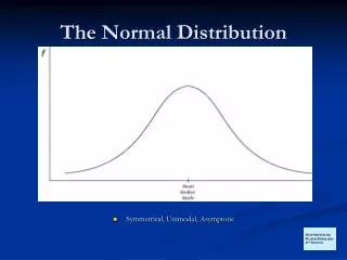
Symmetrical, Unimodal, Asymptotic The Normal Distribution
Frequency Distributions • Many types of distributions • Common Distributions • Normal • T distribution • Uniform • Gamma • Rayleigh • F distribution • Parametric Statistics Assume Normality • Test for normality
Testing for Normality • Skewness and Kurtosis • Histogram Plot with normal distribution curve superimposed • Q-Q Plot • Kolmogorov-Smirnov Test
What if my data is not normal? Nonparametric procedures Log transformation Square root transformation Transform data into categorical variables
Standardization • Standardizing scores is the process of converting each raw score in a distribution to a z score (or standard deviation units) • Raw Score: the individual observed scores on measured variables
X = raw score • = population mean • = standard deviation X = sample mean s = sample standard deviation standard deviation Formula for Calculating z Score OR • Also known as a standard score • Helps to understand where a score lies in relation to other scores on the distribution • Indicates how far above or below the mean a given score in the distribution is in standard deviation units • Calculated using mean and standard deviation OR
The Central Limit Theorem • Central limit theorem: As long as you have a reasonably large sample size (e.g., n≥ 30), the sampling distribution of the mean will be normally distributed (i.e., a bell curve) even if the distribution of scores in your sample is not • the sum of a large number of independent observations from the same distribution has, under certain general conditions, an approximate normal distribution. Moreover, the approximation steadily improves as the number of observations increases.
What is a Standard Error? • A standard error is the standard deviation of the sampling distribution of a given statistic (e.g., the mean, the difference between two means, the correlation coefficient, etc.) • It is the measure of how much random variation we would expect from equally sized samples drawn from the same population • It is the denominator in the formulas used to calculate many inferential statistics
Example: Standard Errors in Depth • Imagine that we wanted to find the average shoe size of adult American women • Suppose we selected a random sample of 100 women from our population. (Measuring the shoe size of all American women is too expensive and tedious.) • Now suppose that we repeat this process of selecting random samples of 100 American women, measuring their shoe sizes, and replacing the sample in the population. • This process of randomly sampling, calculating the mean and returning the members back to the population, is known as sampling with replacement • All the random samples of the population created their own distribution, which is called a sampling distribution of the mean
Standard Errors in Depth (continued) • We can plot sample means in frequency graphs to form distributions of sample means (just like we do with raw scores) • The mean and standard deviation of the sampling distribution of the mean have special names • The mean of the sampling distribution is called the expected value because the mean of the sampling distribution of the means is (or expected to be) the same as the population mean • The standard deviation of the sampling distribution is called the standard error • The standard error of the mean provides a measure of how much error we can expect when we say that a sample mean represents the mean of the larger population (hence, it is called the standard error) Expected value ≈ Population mean Population standard deviation ≈ Standard error
How to Calculate the Standard Error • Since it is costly and difficult to draw several samples from a population, you often must make due with a single sample. Therefore, it is important to examine two characteristics of your sample: • The sample size • The larger the sample, the more likely it will represent the population (if chosen randomly) • The variation of scores within the sample • If scores in the sample are diverse, we can assume that the population is the same, which can reduce our confidence that our sample accurately represents the population Population Sample Sample Sample
How to Calculate the Standard Error • The formula is simply the standard deviation of the sample (or population) divided by the square root of the sample size • Small samples with large standard deviations produce large standard errors • This makes it difficult to have confidence that the sample accurately represents the population • In contrast, a large sample with a small standard deviation will produce a small standard error • This makes it more likely that the sample accurately represents the population OR where = the standard deviation for the population s = the sample estimate of the standard deviation n = the sample size
Sample statistic Standard error The Use of Standard Errors in Inferential Statistics • Inferential statistics: Statistics generated from sample data used to draw conclusions about characteristics of a population from which the sample was drawn • Suppose we want to know whether a relationship that we find between two variables using sample data represents a relationship between the two in the larger population • To answer this question, we need to use standard errors • To summarize, the standard error is used in inferential statistics to see whether our sample statistic is larger or smaller than the average differences (variance or error) in the statistic we would expect to occur by chance.
Sample Size and Standard Deviation Effects on the Standard Error • Suppose we wanted to know the standard error of the mean on the variable “I expect to do well on the test” for each of the two groups in the study, the elementary school students and the middle school students Data collected from a study was examined to compare the motivational beliefs of 137 elementary school students with 536 middle school students • Looking at the Table 6.4, we have the necessary statistics to calculate the standard errors for each sample (i.e., the standard deviations and sample sizes)
Sample Size and Standard Deviation Effects on the Standard Error • Looking at the Table 6.4, the standard deviations look very similar; however, there is a large difference in the two sample sizes • As shown earlier in this chapter, to find the standard error, we simply divide the standard deviation by the square root of the sample size • For the elementary school sample, we need to divide 1.38 by the square root of 137: • Using the same process for the middle school sample, we calculate a standard error of 0.06 • Notice that the standard error of the middle school sample is half the size of the elementary school sample (see next slide) • This difference was due to the difference in sample size, which plays a big role in determining the size of the standard error = = 0.12
Chance, Probability, and Error When making inferences from a sample to a population (as in inferential statistics), there is always some possibility that the sample that was selected from the population does not accurately represent the population. This is where the concepts of chance, probability, and error come into play. • Chance: The probability of a statistical event occurring due simply to random variations in the characteristics of samples of given sizes selected randomly from a population • Error: Also known as random sampling error, this refers to differences between the sample characteristics and the characteristics of the larger population caused merely by random fluctuations, or variability, involved in the process of selecting random samples from a population. When you randomly select two samples of the same size from the same population, you are likely to find differences between these two samples. These differences are due to error, or random sampling error.
Hypothesis Testing A hypothesis establishes a criterion that will be used to decide whether or not a hypothesis should be rejected (e.g., that there is no difference in the driving ability of men and women). • Null Hypothesis (Ho): the hypothesis always suggests that there will be no effect in the population • Alternative Hypothesis (HA or H1): An alternative to the null hypothesis, it claims that there is an effect in the population • An example of a null hypothesis stating that the population mean, µ, will be equal to the mean of the sample: • Ho: µ = • There are two types of alternative hypotheses that can be made. A two-tailed alternative hypothesis does not speculate that a sample is less than or greater than the population, just that it differs. A two-tailed alternative hypothesis claiming that the population mean will not be equal to the sample mean is denoted as: • HA: µ ≠ • A one-tailed alternative hypothesis is a directional claiming that one value will be greater. A one-tailed alternative hypothesis claiming that the population mean will be less than the sample mean is denoted as: • HA: µ <
Type II Error: Failing to reject the null hypothesis when it is actually false To avoid a Type II error a liberal alpha level such as .10 can be used Errors in Hypothesis Testing Before deciding whether to reject or retain the null hypothesis of no effect in the population the researcher must decide how willing he or she is to reject the null hypothesis when it is actually true. In other words, when deciding that an effect in the sample represents a genuine phenomenon in the population, one must conclude that the result was not just due to random sampling error. We can never be certain that a result is not due to random sampling error, so when we reject the null hypothesis we may be wrong. In the sciences we are usually willing to live with an error rate of 5%, so we set an alpha level (α) of .05. If the p value is smaller than the alpha level, the null hypothesis is rejected (see next slide). • Type I Error: Rejecting the null hypothesis when it is actually true • To avoid a Type I error a conservative alpha level like .01 is used.
Graphic Demonstrating Hypothesis Testing for a Two-Tailed Test
Statistical Significance • Statistical significance: the probability (p or p value) that a statistic derived from a sample represents some genuine phenomenon in the population. In other words, the effect observed in the sample data is not due to random sampling error, or chance. • To determine statistical significance, we must compare the size of the effect to our measure of random sampling error, which is usually a measure of standard error.
Effect Size, Statistical Significance, and Practical Significance • The Problem: Because measures of statistical significance rely on the standard error, and the standard error is greatly influenced by sample size, large sample sizes often produce statistically significant results, even for small effects. • Example: Comparing a sample mean of 105 with a population mean of 100, standard deviation of 15, using samples of n =25 and n = 1600: For a 25 person sample: For a 1600 person sample: t = 1.67 t = 13.33 The p value for a t of 1.67 is between .10 and .20 The p value for a t of 13.33 is <.0001
Effect Size, Statistical Significance, and Practical Significance (continued) • The cure: Effect size • To deal with this problem of sample size affecting statistical significance, statisticians calculate effect sizes for their statistics. Effect sizes provide a measure of the statistical effect while minimizing the role of sample size. • The effect size is calculated by essentially removing the sample size from the standard error. This causes the effect to be expressed in standard deviation, rather than standard error, units. • Effect sizes provide a measure of practical significance, using the following guidelines: • d less than .20 is small • d between.25 and .75 is moderate • d greater than .80 is large. • Because practical significance is subjective it is important to take into account the effect size and statistical significance, and understand that it is easier to get chance results form a small sample size than it is from a large sample size
Confidence Intervals • Confidence intervals offer another measure of effect size. By using probability and confidence intervals a researcher can make educated guesses about the approximate value of a population parameter. • Most of the time researchers want to be either 95% or 99% confident that the confidence interval contains the population parameter. Confidence intervals are calculated by:
Confidence Interval Example • Suppose that we have a random sample of 1000 men. We have measured their shoe size and found they have a mean shoes size of 10 with a standard deviation of 2. The standard error of the mean for this sample is .06. Let’s calculate a 95% confidence interval for the population mean. • First, looking in Appendix B for a two-tailed test with df = infinity and α = .05, we find t95 = 1.96. • Plugging this value into our confidence interval formula we, get the following: • CI95 = 10 (1.96)(.06) • CI95 = 10 .12 • CI95 = 9.88, 10.12 “We are 95% confident that the interval between 9.88 and 10.12 contains the population mean.”
Conclusion For several decades, statistical significance has been the measuring stick used by social scientists to determine whether the results of their analyses were meaningful. But tests of statistical significance are quite dependent on sample size. With large samples, even trivial effects are often statistically significant, whereas with small sample sizes, quite large effects may not reach statistical significance. Because of this there has been an increasing appreciation of measures of practical significance. When determining the practical significance of results consider all of the measures at your disposal. Is the result statistically significant? How large is the effect size? How wide is the confidence interval? And in the context of the real world, how important and meaningful is the statistical effect?