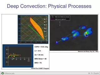
Deep Convection: Physical Processes

1. Deep Convection: Physical Processes M. D. Eastin

2. Deep Convection: Physical Processes • Buoyancy: • Definition, CAPE, and CIN • Maximum Vertical Motion • Effects of Updraft Diameter • Effects of Entrainment • Downdrafts • Vertical Shear: • Hodograph Basics • Estimating Vertical Shear from Hodographs • Hodograph Shape • Estimating Storm Motion from Hodographs • Hodographs and Convective Storm Type • Effects of both Buoyancy and Shear: • Cold Pool – Shear Interactions M. D. Eastin

3. Why Buoyancy and Shear? • Useful Forecast Parameters: • Forecasters must use synoptic observations to anticipate mesoscale weather: • Forecast the likelihood of deep convection • Forecast convective type (single cell, multicell, or supercell) • Forecast convective storm evolution • Forecast the likelihood of severe weather • These mesoscale events can be forecast using common, simple forecast parameters • that incorporate the concepts of buoyancy and shear using observations obtained • from soundings • CAPE and CIN • Lifted Index (LI) • Bulk Richardson Number (BRN) • Storm-Relative Environmental Helicity (SREH) • Energy Helicity Index (EHI) • Supercell Composite Parameter (SCP) • Significant Tornado Parameter (STP) • CAPE/Shear and BRN Phase Spaces • First, let’s examine the basic shear and buoyancy processes, and tools to estimate each… We will cover the application of these forecast parameters in future lectures… M. D. Eastin

4. Buoyancy • Definition of Buoyancy • Force that acts on a parcel of air due to a density difference between the parcel • and the surrounding “environmental” air • The force causes the air parcel to accelerate upward or downward • Buoyancy is a basic process in the generation of all convective updrafts and downdrafts • What physical factors determine a parcel’s buoyancy? • How can we estimate buoyancy from standard observations? • What are limiting factors for those buoyancy estimates? M. D. Eastin

5. Buoyancy • What physical factors determine a parcel’s buoyancy? • Let’s return to basic dynamics and the vertical equation of motion: • For synoptic-scale motions in the free atmosphere the vertical accelerations are small • and friction is negligible • Thus, the equation reduces to hydrostatic equation • Or • Synoptic-scale systems are largely in hydrostatic balance! Vertical Acceleration Vertical PGF Gravity Friction M. D. Eastin

6. Buoyancy • What physical factors determine a parcel’s buoyancy? • On the mesoscale, vertical accelerations can be very large, and thus not in hydrostatic • balance. Also, friction (or turbulent mixing) is no longer negligible, so we now have: • This equation can be re-written as (see Sections 2.3.3 and 3.1 of you book): • where: • Total Buoyancy Force What does each term physically represent? M. D. Eastin

7. Buoyancy and CAPE • What physical factors determine a parcel’s buoyancy? • Thermal Buoyancy: • Temperature difference between an air parcel • and its environment • We estimate the total buoyancy force available to • accelerate an updraft air parcel by computing the • Convective Available Potential Energy (CAPE) • CAPE is the sum of the energy in the positive area CAPE has units of J/kg EL Tenv Tpar LFC CAPE has units of J/kg M. D. Eastin

8. Buoyancy and CIN • What physical factors determine a parcel’s buoyancy? • Thermal Buoyancy: • We can also estimate the total buoyancy force • available to decelerate an updraft air parcel by • computing the Convective Inhibition (CIN) • CIN is the sum of the energy in the negative area • CIN is the result of a capping inversion located • above the boundary layer • Remember: The CIN must be overcome before • deep convection can develop LFC CIN has units of J/kg SFC Methods to overcome CIN: 1. Mesoscale Lifting 2. Near-surface Heating 3. Near-surface Moistening M. D. Eastin

9. Buoyancy and Moisture Effects • What physical factors determine a parcel’s buoyancy? • Moisture Buoyancy: • Specific humidity difference between an air • parcel (often saturated) and its environment • Smaller in magnitude, but not negligible • Can be incorporated into CAPE (and CIN) • by using virtual temperatures (Tv) • This incorporation is NOT always done • When neglected → small underestimation of CAPE • → small overestimation of CIN Remember: M. D. Eastin

10. Buoyancy and Water Loading • What physical factors determine a parcel’s buoyancy? • Water Loading: • Total liquid (and ice) cloud water content (qc) and • rain water content (qr) • Effectively adds weight to the air parcel • Always slows down (decelerate) updrafts • Can be large • Can initiate downdrafts • Difficult to observe → Can be estimated from • radar reflectivity once • storms develop • Always neglected in the CAPE and CIN calculations M. D. Eastin

11. Updraft Velocity • What is a parcel’s maximum updraft velocity? • One reason CAPE is a useful parameter to forecasters is that CAPE is directly related • to the maximum updraft velocity (wmax) an air parcel can attain: • This equation is obtained from a simplified version of the vertical momentum equation • that neglect the effects of water loading, entrainment (mixing), and the vertical • perturbation pressure gradient force (see Section 3.1.1 of your text) • Due to these simplifications, the above equation often over estimates the maximum • vertical motion by a factor of two (2): • Example: → Accounting for the simplifications M. D. Eastin

12. Limiting Factors • Effects of Updraft Diameter: • Any warm parcel produces local • pressure perturbations on the • near environment • A simple mesoscale application • of the hypsometric equation • The positive pressure perturbation • (a relative high pressure) above • the parcel combined with the • negative pressure perturbation • (a relative low pressure) below • the parcel produce a symmetric • overturning circulation that allows • air to move out of the parcel’s path • and then fill in behind the parcel • to maintain mass continuity H H L L H H L L H H L L M. D. Eastin

13. Limiting Factors • Effects of Updraft Diameter: • These pressure perturbations • produce a downward-directed • pressure gradient that opposes • the upward-directed buoyancy • force – slows down the updraft • Wide updrafts (bubbles) • Larger pressure gradients • Slower updrafts • Narrow updrafts (bubbles) • Smaller pressure gradients • Faster updrafts H H L L M. D. Eastin

14. Limiting Factors • Effects of Entrainment: • Entrainment mixing of environmental air into the updraft parcel always decreases • the net buoyancy force acting on the updraft parcel (which reduces wmax) • The vertical distributionof CAPE can have a significant effect on how entrainment • mixing limits updraft strength • Consider two soundings (A and B) • with identical CAPE • Which sounding will produce the • strongest updraft? Why? M. D. Eastin

15. Limiting Factors • Effects of Entrainment: • Entrainment mixing of environmental air into the updraft parcel always decreases • the net buoyancy force acting on the updraft parcel (which reduces wmax) • The vertical distribution of CAPE can have a significant effect on how entrainment • mixing limits updraft strength • Sounding A: • CAPE confined to the lower levels • Updraft will accelerate more quickly, • allowing less time for entrainment • mixing to reduce its net buoyancy • Stronger updraft • Sounding B: • CAPE spread throughout the depth • Slow updraft acceleration allows • more time for entrainment to reduce • the net buoyancy • Weaker updraft M. D. Eastin

16. Limiting Factors • Effects of Entrainment: • Entrainment mixing of environmental air into the updraft parcel always decreases • the net buoyancy force acting on the updraft parcel (which reduces wmax) • The amount of environmental moisture can have a significant effect on how • entrainment mixing limits updraft strength • Consider two soundings (A and B) • with identical distributions of CAPE, • but different environmental moisture • at mid-levels • Which sounding will produce the • strongest updraft? Why? M. D. Eastin

17. Limiting Factors • Effects of Entrainment: • Entrainment mixing of environmental air into the updraft parcel always decreases • the net buoyancy force acting on the updraft parcel (which reduces wmax) • The amount of environmental moisture can have a significant effect on how • entrainment mixing limits updraft strength • Sounding A: • The entrainment of environmental • air will produce some evaporational • cooling, reducing the net thermal • buoyancy • Updraft will weaken some • Sounding B: • Entrainment of environmental air • will produce lots of evaporational • cooling, significantly reducing the • net thermal buoyancy • Updraft will weaken considerably • Downdraft may develop M. D. Eastin

18. Downdrafts • What Processes Produce Downdrafts? • The two primary buoyancy forcing processes that generate downdrafts are water loading and evaporational cooling Water Loading: • Effectively “drags” air parcels down • Forcing magnitude depends on the amount • of water and the initial updraft strength • (strong updrafts can suspend more water) • Difficult to determine or forecast • Evaporational Cooling: • Results from entrainment mixing • Cools air parcels → negative thermal buoyancy • Forcing magnitude depends on the amount of • water available for evaporation and the dryness • of the air into which the water would evaporate • Can determine the maximum cooling a parcel • might experience → wet-bulb temperature M. D. Eastin

19. Downdrafts • Estimating Downdraft Strength: • Air parcels experiencing evaporation will • cool to their wet-bulb temperature (Tw) • (remember sling psychrometers?) • Downdrafts experiencing evaporation will • descend from their wet-bulb temperature • along a moist adiabat, or at a constant • wet-bulb potential temperature (θw) • Represents the coldest temperature • a downdraft parcel could achieve • Similar to updrafts, we estimate the total • buoyancy force available to accelerate a • descending air parcel by computing the • Downdraft Convective Available Potential • Energy (DCAPE) • The maximum downdraft velocity can also • be estimated in a similar manner Evaporation brings parcel to saturation Downdraft originating at 700 mb Tw DCAPE Coldest Possible SFC Temp θw M. D. Eastin

20. Downdrafts • Cold Pool Development: • Besides contributing to downdraft strength, • evaporative processes also contribute to • the development, strength, and speed of • the surface cold pool (and gust front) • Since the cold pool and gust front help • initiate further convection, evaporation • and convective downdrafts are almost • required for long-lived storms • Storms in a very moist environment will • experience minimal evaporation cooling, • weak downdrafts, small cold pools, and • often short lifetimes • Storms in a drier environment experience • moderate evaporational cooling, ample • downdrafts, moderate cold pools, and • often experience long lifetimes • “Catch 22”: A very dry environment is BAD M. D. Eastin

21. Buoyancy Summary • Summary of Buoyancy Processes: • Buoyancy is a fundamental process in the generation and maintenance of all convective • updrafts and downdrafts • Positive contributions to buoyant energy and updraft strength come from potential • temperature and water vapor differences from the large-scale environment • CAPE provides a quantitative estimate of buoyant energy available for updrafts to • accelerate, especially when calculated using an appropriate low-level average of • both moisture and temperature (e.g., the lowest 100mb layer) • • CAPE can be used to estimate updraft strength (wmax) • CIN can either prevent convective storm development entirely or delay initiation until • maximum heating is reached • • Thermodynamic diagrams are the essential tool for estimating the effects of vertical • buoyancy distribution and entrainment on both updraft and downdraft strength • • Downdraft strength depends on both water loading and evaporation processes • • In general, drier mid-levels are associated with stronger downdrafts • DCAPE provides a quantitative estimate of buoyant energy available for downdrafts to • accelerate, and can be used to estimate downdraft strength M. D. Eastin

22. Vertical Shear • Definition of Vertical Shear • The vector difference between the horizontal winds at two levels • The resulting vector is called the “vertical wind shear” • A description of how the horizontal winds change with height • Vertical shear is present in all environments where convective updrafts and downdrafts • occur (ranging from minimal shear to very large shear) • How can we estimate vertical shear • from standard observations? • How does vertical shear modulate • storm structure and evolution? M. D. Eastin

23. Hodograph Basics • A Method to Show Vertical Wind Shear: The Hodograph • A means to convey the vertical profile of winds observed by a sounding (rawindsonde) • Based on observed winds displayed as vectors • Shows structure of vertical shear throughout the troposphere M. D. Eastin

24. Hodograph Basics • How a Hodograph is Constructed • Start with wind observations from a sounding • Use the polar coordinate system (or a polar stereographic grid) • Starting at the origin, plot each wind vector as a function of direction and magnitude • Connect the endpoints of each vector to “form the hodograph” M. D. Eastin

25. Vertical Shear • Estimating Vertical Shear from a Hodograph • The hodograph is actually composed of the vertical wind shear vectors between each layer • The shear magnitude and direction for an individual layer is shown by each yellow arrow • The total shear over a deep layer can be found by summing the length of all shear vectors through the layer (can be done on hodograph – easier with software → Excel) Estimating the shear magnitude for any individual layer Estimating the total shear magnitude through a deep layer Measure the length of all the vectors aligned along an axis Measure the length of any individual shear along an axis M. D. Eastin

26. Vertical Shear • Estimating Vertical Shear from a Hodograph • The hodograph is actually composed of the vertical wind shear vectors between each layer • The shear magnitude and direction for an individual layer is shown by each yellow arrow • The mean shear over some layer can be found by first computing the total shear over that • layer and then dividing by the depth of the layer (more easily done with software → Excel) Estimating the mean shear magnitude through a deep layer Find the total shear, then divide by the layer depth M. D. Eastin

27. Vertical Shear • Estimating Vertical Shear from a Hodograph • The bulk shear through a deep layer can estimated by the following process: • (experienced forecasters can visually estimate – others use software → Excel): • Determine the shear vector for each level • relative to the surface wind (light blue vectors) • Separate these surface-relative shear vectors • into their “u” and “v” components • Compute the mean “u” and “v” through the layer • Combine the mean components back into vector • form to get the bulk shear vector • This four-step process is valid for all hodograph • shapes and sizes • The bulk shear magnitude has been found • to be a good predictor of convective storm type Bulk Shear Vector M. D. Eastin

28. Vertical Shear Distribution • Estimating Vertical Shear from a Hodograph • The distribution of vertical shear through the depth of the hodograph can also have • important implications for convective storm type Total shear = 30 kts Mean shear = 15 kts Shear evenly distributed through the depth Multicells / Squall Lines are more likely Total shear = 30 kts Mean shear = 23 kts Most shear (~23 kts) is confined to the lowest 3 km Supercells / Tornadoes are more likely M. D. Eastin

29. Hodograph Shape • Vertical Shear and Hodograph Shape • The shape of the vertical shear through the hodograph depth can also have important • implications for convective storm type as well as structure and evolution …more on • this later • Important questions: • What is the general hodograph shape? • 1. curved • 2. straight • When does it curve? • 1. throughout the depth • 2. near the surface • 3. only aloft • Through what levels does it curve? • 1. shallow curve • 2. deep curve • What direction does it curve? • 1. clockwise • 2. counter-clockwise M. D. Eastin

30. Hodograph Shape • Vertical Shear and Hodograph Shape • The shape of the vertical shear is influenced by whether speed shear (due to • wind magnitude differences), directional shear (due to directional differences), • or some combination of both speed and directional shear are present Speed Shear Directional Shear M. D. Eastin

31. Hodograph Shape • Vertical Shear and Hodograph Shape • The shape of the vertical shear is influenced by whether speed shear (due to • wind magnitude differences), directional shear (due to directional differences), • or some combination of both speed and directional shear are present Examples of Combined Speed and Directional Shear M. D. Eastin

32. Storm Motion & Storm Relative Flow • Significance of Storm-Relative Flow: • In forecasting storm structure and evolution, a crucial factor is the nature of the storm’s • inflowing air… Will the inflow be warm and moist or cold and dry? • Since most storms move through their environment, one must consider a storm’s inflow • relative to its motion through the environment (i.e. look at the storm-relative flow) • Thus, we first need estimate the expected storm motion from a hodograph so we can • subtract it from the ground-relative winds to obtain the storm-relative winds Ground Relative Winds Storm Relative Winds M. D. Eastin

33. Storm Motion • Estimating Storm Motion from a Hodograph • If storms have already developed → Use radar animations to get storm motion • If storms have not developed → Use hodograph to estimate • Which levels do we use? • Observations and numerical models suggest that most convective storms move with a • velocity close to the 0-6 km AGL mean wind. M. D. Eastin

34. Storm Motion • Estimating Storm Motion from a Hodograph: • Separate the ground-relative winds at each level in to their “u” and “v” components • Compute a mean “u” and a mean “v” • Combine the mean values back into vector form to get the storm motion • This three-step process is applicable to all hodograph shapes and sizes Example component separation for 3–km wind Example Mean Wind Calculation M. D. Eastin

35. Storm-Relative Winds • Estimating Storm-Relative Motions from a Hodograph: • Re-orient the polar grid origin to the computed storm motion • Storm-relative winds are determined by drawing vectors from this new origin to the • shifted hodograph at each level (blue vectors below). • This two-step process is valid for all hodograph shapes and sizes. M. D. Eastin

36. Mean Wind vs. Bulk Shear Difference between the Mean Wind and the Bulk Shear: • Bulk Shear • Relative to the surface wind • Used to estimate storm evolution • (more on this aspect later) • Mean Wind • Relative to the stationary ground • Used to estimate storm motion Mean Shear Vector Mean Wind Vector Stationary ground M. D. Eastin

37. Vertical Shear and Storm Type • Composite Observed Hodographs: • The magnitude and shape of the vertical • shear profile has a strong influence on • convective storm type: • Observed hodographs near deep convection: • Single cells → Weak shear • Multicells → Moderate shear • Supercells → Strong shear Single Cells Multicells Supercells From Chisholm and Renick (1972) M. D. Eastin

38. Vertical Shear and Storm Type • Spectrum of Hodographs and Storm Types: • With the help of a numerical model, Joe Klemp and Morris Weisman (NCAR), documented • how changing only the hodograph shape and shear magnitude can have profound effects • on storm structure: • Klemp and Wilhelmson numerical model • Each simulation has identical initial conditions EXCEPT for the environmental winds • Environmental CAPE = ~2200 J/kg in each simulation • A total of seven (7) simulations • For each simulation the follow information is shown • Hodograph • Rainfall structure (contours) at 1.8 km AGL • Updraft locations (shaded) at 4.6 km AGL • Surface gust front location (cold front) Shown for 40, 80, and 120 min M. D. Eastin

39. Vertical Shear and Storm Type Weak Deep Shear Semicircular Weak Multicell The cold pool gust front “out ran” the convection Convection along gust front Moderate Deep Shear Semicircular Strong Multicell Weak Supercell From Weisman and Klemp (1986) M. D. Eastin

40. Vertical Shear and Storm Type The cold pool gust front out ran the convection Weak Shallow Shear Curved Weak Multicell Convection along gust front Moderate Shallow Shear Curved Strong Multicell M. D. Eastin

41. Vertical Shear and Storm Type Moderate Deep Shear Curved-Straight Two Multicells (Split) Convection along gust front Convection along gust front Moderate Deep Shear Straight Two Supercells (Split) M. D. Eastin

42. Vertical Shear and Storm Type The cold pool gust front out ran the convection Strong Deep Shear Curved-Straight Strong Supercell Weak Multicell (Split) Convection along gust front M. D. Eastin

43. Vertical Shear Summary • Summary of Shear Processes: • Vertical shear is a fundamental process in modulating convective storms • Hodographs are the essential tool for determining the magnitude, direction, and • shape of the environmental and storm-relative vertical wind shear • Storm motion can be estimated from a hodograph as the 0-6 km mean wind • The magnitude and shape of the vertical wind shear has a strong influence on • convective storm type: • Weak shear → Single cells and multicells • Moderate shear → Multicells and supercells • Strong shear → Supercells • Shear over a greater depth increases the likelihood of supercells • Greater curvature increases the likelihood of sueprcells M. D. Eastin

44. Effects of Buoyancy and Shear • Interactions between the Cold Pool and the Vertical Shear : • The numerical simulation results indicated that the stronger and longer-lived • multicell and supercell storms where those that continued to develop deep • convection along the gust front • Storm type, intensity, and longevity are linked to how the cold pool interacts with • the low-level vertical shear to continuously lift parcels to their level of free convection • Let’s examine this process… M. D. Eastin

45. Cold Pool and Shear Interactions • Cold Pool Motion: • The majority of a cold pool’s “forward” • speed (c) is a function of it depth and • its temperature difference from the • environmental air • where: h = cold pool depth • Colder and deeper cold pools move faster • than “warmer” and shallower cold pools • A small portion of a cold pool’s forward motion results from local high pressure produced hydrostatically within the cold air and its down gradient flow M. D. Eastin

46. Cold Pool and Shear Interactions • Cold Pool Circulations: • The spreading cold pool can also be • described in terms of the circulation • found at its leading edge • Vorticity is created at the leading edge • Vorticity can be created by either: • Shear • Tilting • Density (buoyancy) gradients • Horizontal vorticity (η) is generated • when ever there are horizontal • gradients of buoyancy (B): z x M. D. Eastin

47. Cold Pool and Shear Interactions • Cold Pool Circulations: • By itself, the cold pool can only • generate deep convection if the • upward motion on its leading edge • can lift the warm air to its LFC • Because the cold pool circulation • also pulls the warm air back down, • by itself it may not be efficient at • retriggering new cells unless the • LFC is very close to the ground • Now, let’s add vertical wind shear • to the picture M. D. Eastin

48. Cold Pool and Shear Interactions • Shear Circulations: • Vertical shear creates horizontal • vorticity within the ambient • (or environmental) flow • Given westerly vertical wind shear: • What sign will the ambient • horizontal vorticity be? • On which side of the cold • pool will there be deeper • lifting as it interacts with • the vertical wind shear? z x “Upshear” “Downshear” Shear Vector Shear Vector M. D. Eastin

49. Cold Pool and Shear Interactions • Cold Pool – Shear Circulations: • In this example, new cells will be triggered on the east side of the cold pool where the lifting is deeper • The deeper lifting is created by the balance between the cold pool and shear horizontal vorticity • Thus, assessing the low- to mid-level • shear vector is crucial for determining • how a multicell system will propagate Upshear Downshear Shear Vector M. D. Eastin

50. Cold Pool and Shear Interactions • Optimal Interactions: • Optimal vertical lifting will • occur when the cold pool • circulation is of the same • strength as the shear • circulation • (i.e. balanced circulations) • If either the cold pool • or shear circulation is • dominant, then the • warm inflowing air will • be “pulled back” by the • dominant circulation • creating tilted convection • Will be discussed more • when squall lines are • covered in detail • (Section 9.3 in your text) Cool Pool circulation dominates Shear circulation Balanced Cool Pool and Shear Circulations Shear circulation dominates Cold Pool circulation M. D. Eastin