Floating Point Vector Processing using 28nm FPGAs
330 likes | 437 Vues
This paper discusses the innovative techniques presented at the HPEC Conference by Michael Parker and Dan Pritsker from Altera Corp, focusing on the use of 28nm FPGAs for high-performance computing. A novel floating-point methodology optimized for single and double-precision operations is introduced, enabling 1-TFLOP processing capability. Highlights include efficient support for the IEEE 754 format, improved mantissa precision through a fused datapath approach, and QR decomposition algorithm implementation designed for FPGA architecture. The methodologies discussed pave the way for increased performance in floating-point operations.

Floating Point Vector Processing using 28nm FPGAs
E N D
Presentation Transcript
Floating Point Vector Processing using 28nm FPGAs HPEC Conference, Sept 12 2012 Michael Parker Altera Corp Dan Pritsker Altera Corp
28-nm DSP Architecture on Stratix V FPGAs User-programmable variable-precision signal processing Optimized for single- and double-precision floating point Supports 1-TFLOP processing capability 2
Why Floating Point at 28nm ? • Floating point density determined by hard multiplier density • Multipliers must efficiently support floating point mantissa sizes 3.2x 1.4x 6.4x 4x 1.4x 5SGSB8 65nm 40nm 28nm
Floating Point Multiplier Capabilities • Floating point density determined by hard multiplier density • Multipliers must efficiently support floating point mantissa sizes 3.2x 1.4x 6.4x 4x 1.4x 5SGSD8 65nm 40nm 28nm
Floating-point Methodology • Processors – each floating-point operation supports IEEE 754 format • Inefficient format for FPGAs • Not 2’s complement • Special cases, error conditions • Exponential normalization for each step • Excessive routing requirement resulting in low performance and high logic usage • Result: FPGAs restricted to fixed point Denormalize Normalize
New Floating-pointMethodology • Processors – each floating-point operation supports IEEE 754 format • Inefficient format for FPGAs • Not 2’s complement • Special cases, error conditions • Exponential normalization for each step • Excessive routing requirement resulting in low performance and high logic usage • Result: FPGAs restricted to fixed point • Novel approach: fused datapath • IEEE 754 interface only at algorithm boundaries • Signed, fractional mantissa • Increases mantissa precision → reduces need for normalization • Result: 200-250 MHz performance with large complex floating-point designs Slightly Larger – Wider Operands True Floating Mantissa (Not Just 1.0 – 1.99..) Denormalize Normalize Remove Normalization Do Not Apply Special and Error Conditions Here
Vector Dot Product Example + + + + + + + X X X X X X X X Normalize DeNormalize
Selection of IEEE Precisions • IEEE format • 7 precisions (including double and single) • float16_m10 • float26_m17 • float32_m23 (IEEE single) • float35_m26 • float46_m35 • float55_m44 • float64_m52 (IEEE double)
Elementary Mathematical Functions Selectable Precision Floating Point The new fn(pi*x) and fn(x)/pitrig functions are particularly logic efficient when used in floating point designs Highlighted functions are limited to IEEE single and double
QR Decomposition • QR Solver finds solution for Ax=b linear equation system using QR decomposition, where Q is ortho-normal and R is upper-triangular matrix. A can be rectangular. • Steps of Solver • Decomposition: A = Q · R • Ortho-normal property: QT · Q = I • Substitute then mult by QT: Q · R · x = b R · x = QT · b = y • Backward Substitution: QT · b = y solve R · x = y • Decomposition is done using Gram-Schmidt derived algorithms. Most of computational effort is in “dot-product”
Block Diagram Stimulus Backward Substitution QR Decomposition + Q MatrixT * Input Vector [m x n] A R x [m] b y Solve for x in Ax = b where A is non-symmetric, may be rectangular
QR Decomposition Algorithm for k=1:n r(k,k) = norm(A(1:m, k)); for j = k+1:n r(k, j) = dot(A(1:m, k), A(1:m, j)) / r(k,k); end q(1:m, k) = A(1:m, k) / r(k,k); for j = k+1:n A(1:m, j) = A(1:m, j) - r(k, j) * q(1:m, k); end end • Standard algorithm, source: Numerical Recipes in C • Possible to implement as is, but changes make it FPGA friendly and increase numerical accuracy and stability
Algorithm - Observations for k=1:n r(k,k) = sqrt(dot(A(1:m, k), A(1:m,k)); for j = k+1:n r(k, j) = dot(A(1:m, k), A(1:m, j)) / r(k,k); end q(1:m, k) = A(1:m, k) / r(k,k); for j = k+1:n A(1:m, j) = A(1:m, j) - r(k, j) * q(1:m, k); end end k sqrt, k*m cmults k2/2 divides, m*k2/2 cmults k divides m*k2/2 cmults • Replaced norm function with sqrt and dot functions, as they are available as hardware components. • k sqrt • k2/2 + k divides • m*k2 complex mults
Algorithm - Data Dependencies for k=1:n r(k,k) = sqrt(dot(A(1:m, k), A(1:m,k)); for j = k+1:n r(k, j) = dot(A(1:m, k), A(1:m, j)) / r(k,k); end q(1:m, k) = A(1:m, k) / r(k,k); for j = k+1:n A(1:m, j) = A(1:m, j) - r(k, j) * q(1:m, k); end end r(k,k) required at this stage r(k,k) required at this stage q(1:m,k) required at this stage • Floating point functions may have long latencies • Dependencies introduce stalls in data flow • Neither r(k,j) nor q can be calculated before r(k,k) is available • A(1:m,j) cannot be calculated before q is available
Algorithm - Splitting Operations for k=1:n %% r(k,k) = sqrt(dot(A(1:m, k), A(1:m,k)); r2(k,k) = dot(A(1:m, k), A(1:m,k); r(k,k) = sqrt(r2(k,k)); for j = k+1:n %% r(k, j) = dot(A(1:m, k), A(1:m, j)) / r(k,k); rn(k, j) = dot(A(1:m, k), A(1:m, j)); r(k, j) = rn(k,j)/ r(k,k); end q(1:m, k) = A(1:m, k) / r(k,k); for j = k+1:n A(1:m, j) = A(1:m, j) - r(k,j) * q(1:m,k); end end
Algorithm - Substitutions for k=1:n r2(k,k) = dot(A(1:m, k), A(1:m,k); r(k,k) = sqrt(r2(k,k)); for j = k+1:n rn(k, j) = dot(A(1:m, k), A(1:m, j)); r(k, j) = rn(k,j)/ r(k,k); end q(1:m, k) = A(1:m, k) / r(k,k); for j = k+1:n A(1:m, j) = A(1:m, j) - r(k,j) * q(1:m,k); end end Replace q(1:m,k) with A(1:m,k) / r(k,k) Replace r(k,j) with rn(k,j)/ r(k,k)
Algorithm - After Substitutions for k=1:n r2(k,k) = dot(A(1:m, k), A(1:m,k); r(k,k) = sqrt(r2(k,k)); for j = k+1:n rn(k, j) = dot(A(1:m, k), A(1:m, j)); r(k, j) = rn(k,j)/ r(k,k); end q(1:m, k) = A(1:m, k) / r(k,k); for j = k+1:n A(1:m, j) = A(1:m, j) - rn(k,j)/ r(k,k) * A(1:m,k) / r(k,k); end end
Algorithm - Re-Ordering for k=1:n r2(k,k) = dot(A(1:m, k), A(1:m,k); for j = k+1:n rn(k, j) = dot(A(1:m, k), A(1:m, j)); end for j = k+1:n A(1:m, j) = A(1:m, j) – (rn(k,j) / r2(k,k)) * A(1:m,k); end end for k=1:n r(k,k) = sqrt(r2(k,k)); for j = k+1:n r(k, j) = rn(k,j)/ r(k,k); end q(1:m, k) = A(1:m, k) / r(k,k); end
Algorithm - Flow Advantages for k=1:n r2(k,k) = dot(A(1:m, k), A(1:m,k); for j = k+1:n rn(k, j) = dot(A(1:m, k), A(1:m, j)); end for j = k+1:n A(1:m, j) = A(1:m, j) - rn(k,j) * A(1:m,k) / r2(k,k); end end for k=1:n r(k,k) = sqrt(r2(k,k)); for j = k+1:n r(k, j) = rn(k,j)/ r(k,k); end q(1:m, k) = A(1:m, k) / r(k,k); end No sqrt Less operations in critical path calculation of “A” Split out: Operations can be scheduled as data becomes available
Algorithm - Number of Calculations k*m complex mults for k=1:n r2(k,k) = dot(A(1:m, k), A(1:m,k); for j = k+1:n rn(k, j) = dot(A(1:m, k), A(1:m, j)); end for j = k+1:n A(1:m, j) = A(1:m, j) – (rn(k,j)/r2(k,k)) * A(1:m,k); end end for k=1:n r(k,k) = sqrt(r2(k,k)); for j = k+1:n r(k, j) = rn(k,j)/ r(k,k); end q(1:m, k) = A(1:m, k) / r(k,k); end m*k2/2 complex mults k2/2 divides, m*k2/2 complex mults k sqrts k2/2 divides k divides • k sqrt • k2 + k divides - twice as many as original, but still only 1 divider per m complex mults • m*(k2+k) complex mults
QRD Structure Ak v A mult/add unit div/sqrt unit m/v m n control Addresses, instructions rk,j r2k,k Fifo (“leaky bucket”)
Running the Design • Initialization feedback in Matlab window
Running the Design • After simulation run analyze_DSPBA_out.m
Computational error analysis Using Single Precision Floating Point