Download
1 / 37
370 likes | 496 Vues
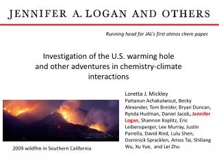
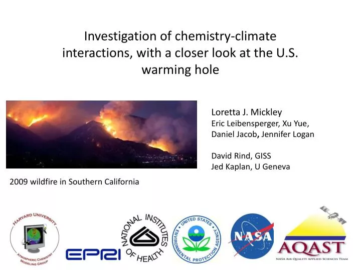
Investigation of chemistry-climate interactions, with a closer look at the U.S. warming hole. Loretta J. Mickley Eric Leibensperger , Xu Yue , Daniel Jacob , Jennifer Logan David Rind , GISS Jed Kaplan , U Geneva. 2009 wildfire in Southern California.

E N D
Investigation of chemistry-climate interactions, with a closer look at the U.S. warming hole Loretta J. Mickley Eric Leibensperger, XuYue, Daniel Jacob,Jennifer Logan David Rind, GISS JedKaplan, U Geneva 2009 wildfire in Southern California
Millions of people in US live in areas with unhealthy levels of ozone or particulate matter (PM2.5). Number of people living in areas that exceed the national ambient air quality standards (NAAQS) in 2010. Ozone daily maximum 8-hour average PM2.5 24-hour average or annual average Bars on barplot will change with changing emissions. Climate change could also change the size of these bars, by changing the day-to-day weather.
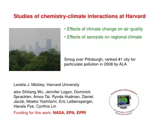
Black carbon California fire plumes Pollution off U.S. east coast Particles affect solar radiation directly…and also indirectly by modifying cloud properties. Light-colored particles reflect sunlight and cool the earth’s surface. Aircraft contrails and cirrus over Europe cooler
VOCs -- volatile organic compounds NH3 -- ammonia . . . . . . SO2 -- sulfur dioxide NOx -- nitrogen oxides Life cycle of particulate matter (PM, aerosols) ultra-fine (<0.01 mm) fine (0.01-1 mm) cloud (1-100 mm) precursor gases nucleation cycling coagulation condensation Soup of chemical reactions coarse (1-10 mm) Organic carbon scavenging Black carbon SO2 SO2 VOCs NOx NOx VOCs NOx NH3 VOCs NOx VOCs NOx combustion volcanoes agriculture biosphere sea salt wildfires combustion dust
Model frameworks 1. Standard Assimilated meteorology GEOS-4 GEOS-5 Atmospheric Chemistry GEOS-Chem 2. Chemistry-climate Chemical feedbacks Meteorology from freely running climate model Atmospheric Chemistry GEOS-Chem Land cover model Fire prediction model
Climate change Air Quality • Wildfire in the western United States in the mid-21st century • Consequences for air quality. Rim fire, Yosemite Natl Park, 2013
Effects of wildfires on air quality in cities in Western US can be very dramatic. • Hayman fire, June 8-22, 2002 • 56,000 ha burned • 30 miles from Denver and Colorado Springs Unhealthy air quality in Denver June 9, 2002 June 8, 2002 PM10 = 372 μg/m3 PM2.5 = 200 μg/m3 Standard = 35 µg/m3 PM10 = 40 μg/m3 PM2.5 = 10 μg/m3 Colorado Dept. of Public Health and Environment Vedal et al., 2006
Fire activity had a big impact on California air quality in 2013. Rim Fire Timeseries of 3-hour average PM2.5 concentrations in Foothills Area Hazardous levels > 250 mg m-3 PM2.5 (mg m-3) Very unhealthy Aug 28 August 31 August 20 Will fire change in the future climate? Unhealthy air Very unhealthy air Aug 30
Observations suggest that fires are increasing in North America. Area burned in Canada has increased since the 1960s, correlated with temperature increase. obs temperature area burned Gillett et al., 2004 5 yr means 1960 2000 Increased fire frequency over the western U.S. since 1970, related to warmer temperatures and earlier snow melt. 1970 2000 Westerling et al., 2007
IPCC AR4 models show increasing temperatures across North America by 2100 in A1B scenario. D Temperature JJA, oC D Precipitation JJA, % Number of models showing increased precipitation. most models Models show increases of JJA temperatures of ~ 3K in Western US. Results for precipitation changes are not so clear. few models IPCC, 2007
How do we predict fires in a future climate?We don’t have a good mechanistic approach for modeling wildfires. Start with the past. 2 approaches Use ensemble of climate models to gain confidence in prediction. + JJA Temperature increase by 2100 Relationship between observed meteorology + area burned Future area burned Future meteorology
Regression approach. Regress meteorological variables and fire indexes onto annual mean area burned in each of six ecoregions with a stepwise approach. ERM RMF PNW NMS Identify the meteorological variables and fire indexes that best predict area burned. Include lagged met variables. CCS DSW Ecoregions are aggregates of those in Bailey et al. (1994) For example, Area burned in Nevada/ semi-desert = f ( + T summer max that year + RH and rainfall previous years) Best predictors: Temp, RH, precip, Build-up Index, Drought code, Duff moisture code.
Predicted fires match observed area burned reasonably well. Least best fit is in Southern California. Obs Fit RMF ERM PNW NMS CCS DSW Area burned in many ecoregions depends on previous year’s relative humidity, rainfall, or temp. Yue et al., 2013
Start with the past. + Relationship between observed meteorology + area burned Future area burned Future meteorology
Use of an ensemble of 15 climate models improves confidence in the results. • Changes in 2050s climate in the West. • Temperature increases 2-2.5 K. • Changes in precip and relative humidity are small and not always robust. • Next step: apply meteorology from climate models to the two fire prediction schemes. Yue et al., 2013
Wildfire area burned increases across the western United States by the 2050s timeframe. Results from regressions approach. Shown are median results. Yue et al., 2013 + Relationship between observed meteorology + area burned Future area burned Future meteorology
Predicted area burned shows large increases in 2050s during peak months. Units = 104 hectares future present-day X2 increase X4 increase Yue et al., 2013
How will changing area burned affect air quality? Ensemble of climate models Median area burned Emissions = area burned x fuel consumption x emission factors Future meteorology GEOS-CHEM Global chemistry model Future air quality
Organic particles increase in future atmosphere over the western U.S. in summer, especially during extreme events. Cumulative probability of daily mean concentrations of OC, Rocky Mountains D Organic Carbon, OC May-Oct Ma 2050s doubling Present-day JJA Change in summertime mean organic PM2.5 in ~2050s, relative to present-day. Wildfires may swamp efforts to regulate air quality in future. Yue et al., 2013
What do these increases in wildfire aerosol mean for human health? % area burned % OC particles Ongoing project with Yale will look at health impacts of these increases. Yue et al., 2013
How will wildfire change in a changing climate in Canada? Ratio of 2050s area burned to present-day Alaska Boreal Cordillera • Area burned increases in the West due to: • Higher temperatures • More frequent blocking high pressure systems. • Increased rainfall in Central and eastern Canada blunt these effects. Ratio of 2050s area burned to present-day Ecoregions West to East Yue, in progress
Aerosols Climate change • Regional climate effects of 1950-2050 trends in US anthropogenic aerosols. Pittsburgh, 1973
What caused the U.S. warming hole of the 20th century? Observed US surface temperature trend 1 No trend between 1930 and 1980. Warming trend after 1980 0 -1 Contiguous US Observed spatial trend in temperatures, 1930-1990 o C GISTEMP 2010 -1 1
1950 1960 1970 1980 1990 2001 Clearing trend in particles over United States since 1980s suggests possible recent warming. Calculated trend in surface sulfate concentrations Increasing sulfate from 1950-1990s. Decreasing sulfate by 2001. Circles show observations. Leibensperger et al., 2012a
We first perform a pilot study: Constant aerosols vs. zeroed US aerosols Constant aerosols everywhere Spin-up GISS climate model A1B scenario of greenhouse gases Zeroed US aerosols, constant elsewhere 2010 2050 Forcing due to aerosol removal over US Model setup causes large warming over East. By comparison, global DF from CO2 is +1.8 Wm-2.
Results from pilot study: Removal of aerosol sources over US increases annual mean surface temperatures by 0.5 o C. Additional warming due to zeroing of US aerosols Warming due to 2010-2050 trend in greenhouse gases. Summertime temperatures increase as much as 1.5 oC. Only direct aerosol effect included. white areas = insignificant differences Mickley et al., 2012
Warming begins immediately and persists through the decades. D Temperature, 2050s A1B Daily max T Daily mean T Change in surface temperatures due to aerosol removal, Northeast US Warming due to aerosol removal is strongest in late summer / early fall Heatwaves show 1-2 K increase. Mickley et al., 2012
D D Climate response of Northeast to aerosol removal Increased diurnal temperature range, higher Tmax Daily max T Daily mean T Warming, especially in late summer, early fall. D D Shift from increased latent flux to increased sensible and LW flux in late summer. Sensible heat Increased solar flux in July-October Latent heat LW D D Reduced cloud cover and relative humidity Low cloud cover Increased sunlight depletes soil moisture by late summer. Rel humidity
Feedbacks involving soil moisture and low cloud cover amplify local temperature response in Aug-Oct period. D Soil moisture depletes through summer. Cloud cover diminishes in response. Shift from increased latent flux to increased sensible and LW flux in late summer. Sensible heat Latent heat LW Diffuse warming Local warming
1950 1960 1970 1980 1990 2001 Next, we perform a more realistic set of simulations, with changing emissions, 1950-2050. Calculated trend in surface sulfate concentrations Increasing sulfate from 1950-1990s. Decreasing sulfate beginning in 1990s. We applied decadal trends in anthropogenic aerosol to the GISS climate model. Circles show observations. Leibensperger et al., 2012a
Forcing from US anthropogenic aerosols peaks in 1980 -1990s. Direct radiative forcing Forcings over Eastern US Peak forcings -2 W m-2, mainly from sulfate. Warming from black carbon offsets the cooling early in the record. Results suggest little climate benefit to reducing black carbon sources in US. Indirect radiative forcing from clouds is about the same magnitude as direct effect. Net DF Indirect radiative forcing Leibensperger et al., 2012a.
Cooling from U.S. anthropogenic aerosols during 1970-1990. Results are from two 5-member ensembles, with and without US anthropogenic aerosols. Indirect + direct effects included. Cooling is greatest over the Eastern US and North Atlantic. 1 oC cooling at surface over East C Leibensperger et al., 2012b
D Model Temperature 1970-1990 Cooling over U.S. is not co-located with aerosol burden. Local changes in cloud cover and soil moisture amplify the cooling effect. Cooling over North Atlantic strengthens Bermuda High, increasing onshore flow of moisture from Gulf of Mexico. Results are controversial. C D Cloud Cover D Soil moisture availability % %
Observations show intensification of the Bermuda High during the 1980s and early 1990s, apparently consistent with aerosol loading. 1948-1977 1978-2007 Variation of western edge of Bermuda High during JJA, 1948-2007. Edge = 1560-gpm contour line at 850 hPa. Shift westward Westward extent of Bermuda High ERA East NCEP Reference longitude What about effect of Pacific Decadal Oscillation? West Period of greatest aerosol loading 1950 2000 1980 Li et al., 2011
Inclusion of US anthropogenic aerosols improves match with observed trends in surface temperatures over the East. Eastern US • Results suggest that US anthropogenic aerosols can explain the “warming hole.” • Warming since 1990s can be attributed to reductions in aerosol sources. Model without US aerosols Standard model Observations Most of the warming from reducing aerosol sources has already been realized. Leibensperger et al., 2012b
How have competing trends in BC and SO2 over 20th century affected regional climate across mid-latitudes? Timeseries of US emissions BC U.S. SO2 emissions (Tg S) U.S. BC emissions (Tg C) • Ongoing work. • BC aerosol • warms mid- to upper troposphere • cools surface • stabilizes atmosphere • Sulfate cools surface, may augment stabilization. • We will compare model BC with lake core sediments from Adirondacks (Husain et al., 2008) and with ice cores from J. McConnell. SO2 1850 1950 2000 1900 Deposition in Adirondacks obst observations BC deposition (g m-2 a-1) model 1860 1940 Leibensperger, Cusworth, and Mickley
Take home messages. • Area burned by wildfires may increase significantly across western North America by 2050s, depending on the ecosystem. • Increased smoke from wildfires may thwart efforts to regulate air quality in coming decades. This is a climate penalty. • Decreases in aerosol loading may have unintended consequences for regional climate, leading to warming. Wildfires in Quebec the same day. Haze over Boston on May 31, 2010