Download
1 / 36
360 likes | 654 Vues
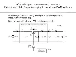
AC modeling of quasi-resonant converters Extension of State-Space Averaging to model non-PWM switches. Use averaged switch modeling technique: apply averaged PWM model, with d replaced by µ Buck example with full-wave ZCS quasi-resonant cell:. µ = F. 7.3. State Space Averaging.

E N D
AC modeling of quasi-resonant convertersExtension of State-Space Averaging to model non-PWM switches Use averaged switch modeling technique: apply averaged PWM model, with d replaced by µ Buck example with full-wave ZCS quasi-resonant cell: µ = F
7.3. State Space Averaging • A formal method for deriving the small-signal ac equations of a switching converter • Equivalent to the modeling method of the previous sections • Uses the state-space matrix description of linear circuits • Often cited in the literature • A general approach: if the state equations of the converter can be written for each subinterval, then the small-signal averaged model can always be derived • Computer programs exist which utilize the state-space averaging method
7.3.1. The state equations of a network • A canonical form for writing the differential equations of a system • If the system is linear, then the derivatives of the state variables are expressed as linear combinations of the system independent inputs and state variables themselves • The physical state variables of a system are usually associated with the storage of energy • For a typical converter circuit, the physical state variables are the inductor currents and capacitor voltages • Other typical physical state variables: position and velocity of a motor shaft • At a given point in time, the values of the state variables depend on the previous history of the system, rather than the present values of the system inputs • To solve the differential equations of a system, the initial values of the state variables must be specified
State equations of a linear system, in matrix form A canonical matrix form: State vector x(t) contains inductor currents, capacitor voltages, etc.: Input vector u(t) contains independent sources such as vg(t) Output vector y(t) contains other dependent quantities to be computed, such as ig(t) Matrix K contains values of capacitance, inductance, and mutual inductance, so that K dx/dtis a vector containing capacitor currents and inductor winding voltages. These quantities are expressed as linear combinations of the independent inputs and state variables. The matrices A,B, C, andE contain the constants of proportionality.
Example State vector MatrixK Input vector Choose output vector as To write the state equations of this circuit, we must express the inductor voltages and capacitor currents as linear combinations of the elements of the x(t) and u( t) vectors.
Circuit equations Find iC1 via node equation: Find iC2 via node equation: Find vL via loop equation:
Equations in matrix form The same equations: Express in matrix form:
Output (dependent signal) equations Express elements of the vector y as linear combinations of elements of x and u:
Express in matrix form The same equations: Express in matrix form:
7.3.2. The basic state-space averaged model Given: a PWM converter, operating in continuous conduction mode, with two subintervals during each switching period. During subinterval 1, when the switches are in position 1, the converter reduces to a linear circuit that can be described by the following state equations: During subinterval 2, when the switches are in position 2, the converter reduces to another linear circuit, that can be described by the following state equations:
Equilibrium (dc) state-space averaged model Provided that the natural frequencies of the converter, as well as the frequencies of variations of the converter inputs, are much slower than the switching frequency, then the state-space averaged model that describes the converter in equilibrium is where the averaged matrices are and the equilibrium dc components are
Solution of equilibrium averaged model Equilibrium state-space averaged model: Solution for X and Y:
Small-signal ac state-space averaged model where So if we can write the converter state equations during subintervals 1 and 2, then we can always find the averaged dc and small-signal ac models
Relevant background • State-Space Averaging: see textbook section 7.3 • Averaged Circuit Modeling and Circuit Averaging: see textbook section 7.4
Averaged Switch Modeling • Separate switch elements from remainder of converter • Remainder of converter consists of linear circuit • The converter applies signals xT to the switch network • The switch network generates output signals xs • We have solved for how xs depends on xT
Block diagram of converter Switch network as a two-port circuit:
The circuit averaging step To model the low-frequency components of the converter waveforms, average the switch output waveforms (in xs(t)) over one switching period.
Relating the result to previously-derived PWM converter models: a buck is a buck, regardless of the switch We can do this if we can express the average xs(t) in the form
Finding µ: ZCS example where, from previous slide,
Derivation of the averaged system equationsof the resonant switch converter Equations of the linear network (previous Eq. 1): Substitute the averaged switch network equation: Result: Next: try to manipulate into same form as PWM state-space averaged result
Conventional state-space equations: PWM converter with switches in position 1 In the derivation of state-space averaging for subinterval 1: the converter equations can be written as a set of linear differential equations in the following standard form (Eq. 7.90): These equations must be equal: Solve for the relevant terms: But our Eq. 1 predicts that the circuit equations for this interval are:
Conventional state-space equations: PWM converter with switches in position 2 Same arguments yield the following result: and
Manipulation to standard state-space form Eliminate Xs1 and Xs2 from previous equations. Result is: Collect terms, and use the identity µ + µ’ = 1: —same as PWM result, but with d µ
Perturbation and Linearization The switch conversion ratio µ is generally a fairly complex function. Must use multivariable Taylor series, evaluating slopes at the operating point:
Small signal model Substitute and eliminate nonlinear terms, to obtain: Same form of equations as PWM small signal model. Hence same model applies, including the canonical model of Section 7.5. The dependence of µ on converter signals constitutes built-in feedback.
Salient features of small-signal transfer functions, for basic converters
µ = F Example 1: full-wave ZCSSmall-signal ac model Averaged switch equations: Linearize: Resulting ac model:
Low-frequency model Tank dynamics occur only at frequency near or greater than switching frequency —discard tank elements —same as PWM buck, with d replaced by F
Example 2: Half-wave ZCS quasi-resonant buck Now, µ depends on js:
Small-signal modeling Perturbation and linearization of µ(v1r, i2r, fs): with Linearized terminal equations of switch network:
Predicted small-signal transfer functionsHalf-wave ZCS buck Full-wave: poles and zeroes are same as PWM Half-wave: effective feedback reduces Q-factor and dc gains