Download
1 / 50
500 likes | 657 Vues
Biomedical Imaging II. Class 6 – Optical Tomography II: Instrumentation 03/13/06. Measurement principle. Measure optical intensity migrating from small irradiation spot ( source , S) to detector (D) position “Scan” object to obtain measurements for many S-D pairs

E N D
Biomedical Imaging II Class 6 – Optical Tomography II: Instrumentation 03/13/06
Measurement principle • Measure optical intensity migrating from small irradiation spot (source, S) to detector (D) position • “Scan” object to obtain measurements for many S-D pairs • Light propagation is scatter-dominated • Signals are obtained under any angle • Signal is strongest near source (backscattered)
DOT characteristics summary • Functional imaging method • Sensitive to hemoglobin oxygenation states (contrast mechanism) • Low spatial resolution (~mm - ~cm) • Excellent temporal resolution (~ms), capability of studying hemodynamics DOT assesses tissue function rather than providing an accurate image of anatomical features. Examples: breast cancer, functional brain imaging
Continuous Wave (C.W.) Measurements • Simplest form of OT: lowest spatial resolution, “easy” implementation, greatest penetration • Measuring transmission of constant light intensity (DC) • Simple, least expensive technology most S-D pairs • High “frame rates” possible
Scalp Bone CSF Cortex Example: Optical brain imaging • “Partial view” or back reflection geometry Source / Detector 1 Detector 2 2-3 cm Detector 3
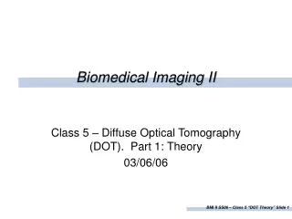
I I t t t0 t0 Time-Resolved Measurements • Measuring the arrival time/temporal spread of short pulses (<ns) due to scattering & absorption (narrowing the “banana”) • Expensive, delicate hardware (single-photon counters, fast lasers, optical reflections, delays…) • Long acquisition times (low frame rates) • Potentially better spatial resolution than DC measurements Prompt or ballistic Photons (t = d/c) “Snake” Photons Diffuse Photons d
I I t t0 t t0 I I Modulation Phase t t t0 t0 Frequency-Domain Measurements • Propagation of photon density waves (PDW): PDW = 9 cm, cPDW = 0.06 c (* • Measure PDW modulation (or amplitude) and phase delay • RF equipment (100MHz-1GHz) • Wave strongly damped, challenging measurement Photon density waves (* f = 200 MHz, μa = 0.1 cm-1, μs’ = 10 cm-1 n = 1.37
Principle components of a DOT system Timing, control DAQ storage Delivery Collection Detector Light source Detector scan Source scan Target
Multi-detector implementation • Scanning of single detector (only used in lab setups): • Safes hardware components, cost • Long acquisition times • Parallel multi-detector acquisition • No “time skew” • Stable setup • Added hardware • Mixed approach (Scanning limited number of detectors) • Feasible for “static imaging” • Used in TR, FD methods because of expensive detection hardware
Multi-source position implementation • Time-division multiplexing : One source position is illuminated at one time for the duration of the detection (~10-100 ms). • Time skew between sources • Switching mechanism necessary: • Optical switch (challenges: isolation, stability, size) • Electronic switching of multiple sources (multiple laser sources & drivers – cost, complexity) • Frequency encoding: All sources are on at the same time. • Intensity modulation at different frequencies allows electronic separation of the signals originating from different sources. • No time skew • Reduced dynamic range
Dynamic range • Ratio of largest to smallest “useable” signal (saturation limit noise limit) • Typically 1:104 (80 dB) for detection electronics • Signal falls of rapidly (~ factor 10 per cm distance on surface) • Determines the maximum tissue volume that can be probed One source With second source
S2 0 1 100 100 1,000 1,000 10 10 1 1 10,000 10,000 100 100 100 1,000 1,000 1,000 0 1 10 10 10 1 1 1 10,000 10,000 10,000 100 100 1,000 1,000 0 10 10 1 1 1 10,000 10,000 100 100 1,000 1,000 10 10 0 1 1 1 10,000 10,000 100 1,000 10 0 1 1 10,000 Solution: Detector gain switching S1 I1
Conduction band Free electrons - Eg < 5 eV for insulator Eg1 eV for semiconductor Eg = 0 eV for metals Electron energy Valence band Bound electrons + Semiconductors I • Energy levels in solids have band structure : • Thermal excitation creates intrinsic carriers (electron-hole pairs): ni = np 1.51010 cm-1 (Si at room temperature, kT = 0.025 eV) • Photoelectric excitation possible for
DEd DEa Semiconductors II • Doping with impurities increases number of free carriers (~ typ. by factor of 107) according to Ea,d 0.045 < kT • Donor: Pentavalent impurity (e.g., P) provides excess e- n-type semiconductor • Acceptor: Trivalent impurity (e.g., B) “captures” e- creates additional holes p -type semiconductor • Internal photoelectric effect: Donor doped: n-type Acceptor doped: n-type
Photodiodes (PD) Positive net charge Negative net charge Diode junction of p-type and n-type semiconductors: • Diffusion of carriers potential across junction (n-type is left positively charged, p-type is left negatively charged) • Recombination at junction region of depletion of free carriers high resistance voltage drop • Carriers generated within diffusion length of the depletion region are separated by potential slope • Photoelectric current Ipproduced by photodiode (proportional to irradiation intensity) Diffusion length + - - + - + + - + - - + - - + - - + + - + - p n + + Ip Cathode Anode
Photodiode (Transimpedance) Amplifier • Converts photocurrent to voltage according to: • Bandwidth: • Highly linear • “Photovoltaic Mode” PD
Photomultiplier tubes (PMT) • External photoelectric effect converts light intensity into current of free electron • Cascade of secondary electron emission / multiplication • Signal amplification G = N typ. ~106 (N: no. of dynodes, : gain per dynode ~4)
Avalanche Photodiodes • Reverse biased with high voltage (~100V) • Internal 10-1000× amplification through avalanche effect • Gain temperature sensitive -> requires cooling/regulation • Available in ready-to-use modules • Pricey
Light sources I • Near infrared range (600-900 nm) • Power ~1-100 mW: Signal quality vs. exposure limit (~ mW/mm2) • Laser diodes (semiconductor lasers): Most widely used • Small • Inexpensive (o.k…. ~$10 - $1000) • High efficiency, easy-to-operate • RF modulation possible • ps-pulsed systems available • (Poor beam quality) • Discrete wavelengths (760, 785, 800, 810, 830,.. nm)
Semiconductor-based light sources • “Forward bias” causes reduction of potential wall diode in conducting mode • Electrons and holes recombine in depletion layer, carriers are replenished by current source • Emitting of recombination radiation light emitting diode • For special diode geometries and reflecting end faces, laser action can be achieved laser diode + - - + - + + - + - - + - - + - - + + p - n + - + + + - - - - - - - - - - - - - + + + + + + + + + + + + + + + + LD LED
Types of laser diodes “5-mm can / 9-mm can:” Low / mid-power (mW-100 mW) Telco app. Hi-power (~W) “Butterfly” “TO3” “HHL” “Fiber pigtail” “C-mount” Hi-power (~W)
Laser diode drivers • Laser diodes require a controlled current source • LD are highly sensitive to ESD, short pulses, and all kinds of electromagnetic interference • Line filters • Power on ramping • Off shorting • LD require cooling and often temperature control to stabilize the output power Thermoelectric cooling (TEC) elements
Light sources II • Solid state lasers: Optically active crystals (TiSa) • Short pulses (< ps, time-resolved systems) • Good beam profile • Bulky (requires pump laser) • Expensive • Difficult to operate • Non-laser sources: light emitting diodes (LED) • Broad wavelength range • Diffuse emitter • Power ~ 10mW
Light propagation in optical fibers I • Snells’ law: • Total internal reflection for a > ac when going from n1 to n2 < n1: • Fiber components: • Core (n1) • Cladding (n2) • Coating (mechanical stab.) • n1 > n2 “guided modes” 0 1
Light propagation in optical fibers II • Acceptance angle a: Maximum incoupling angle ai resulting in guided transmission: • “Numerical Aperture” NA = sina • Divergence angle: Maximum exiting angle ad (aiad aa)
Properties of some optical materials • Important interfaces • Various fiber materials
Fiber modes • Different modes of optical propagation = different spatial intensity patterns • Number of possible modes depending on core radius, refractive indices • Multimode (MM) fibers large core > 50 m • Higher efficiency • Higher power • (Cheaper) • Single-mode (SM) fibers small core < 10 m • Better beam quality • No pulse shape distortion (Telecom apps)
Fiber transmission losses • Absorption losses • Bending losses
Coupling light into optical fibers • Focusing optics must provide: • Focus spot size s core diameter • Beam convergence angle acceptance angle • Mechanical alignment: • Focus on fiber core front face (x-y-z) • Beam perpendicular to front face (-) • Fiber face cut, polished
6 2 4 7 13 3 5 12 1 8 9 11 10 DYNOT system (best DOT imager around!!!)
Fiber Optics • Deliver light to/from tissue • Bifurcated design ( co-located S/D pairs) Probing end Soft jacket Reinforced jacketing Detector fiber bundle Source fiber bundle Bifurcation
Laser Diodes Electrical connectors 830 nm 780 nm Laser Diodes “Fiber pigtails” = opt. output
Commercial Newport 8000 Laser diode and temperature controller Thorlabs Inc. OEM laser driver Laser Controller
Fast Multi-Channel Optical Switch fiber pigtails • Multi-wavelength • 32 fibers • ~70 Hz switch speed = 2Hz frame rate @ 30 sources beam- splitter cube incoupling unit focusing optics circular fiber array rotating mirror source fiber bundles DC servomotor
Multi-Channel Detector • Gain switching • 32 Parallel detection channels • Electronic wavelength separation • Gain Setting of detector determines its sensitivity S/H Gain (TTL) Ref. f2 ´ 1 ´ 1 ´ 1000 ´ 1000 Out @ l2 SiPD Lock-in @ f2 S/H Lock - in S/H @ f2 PTIA PGA Out @ l1 Lock-in @ f1 S/H Lock - in S/H @ f1 PTIA PGA Ref. f1
5 5 6 4 4 9 6 8 3 3 2 2 7 1 1 5 The DYNOT (DYnamic Near-infrared OT) Instrument 1 – power supply, 2 – motor controller, 3 – detector, 4 – laser controller, 5 – host PC w/ monitor, 6 – fiber optics, 7 – optical switch, 8 – optics shielding cover, 9 – laser diodes
Helmet kit can be configured depending on application Probes individually spring loaded Helmet
Measurement Geometries 1 3 4 • Unilateral temporal arrangement (motor cortex) • Distributed Arrangement (frontal, temporal, parietal) • Installing / adjusting the optical probes • Complete 56 arrangement 30 sources 30 detectors = 900 data channels 2
Dual Breast Measurement Head • Patient in prone position • Simultaneous dynamic bilateral breast imaging • Fiber protrusion individually adjusted (manually; pneumatic possible) • Measuring cup positions individually adjusted
Animal Imaging Studies Optical Fibers