Download
1 / 61
610 likes | 911 Vues
Biomedical Imaging. Outline . Biomedical Imaging Images by various imaging modalities Fundamental concepts on imaging Image analysis by MATLAB: analysis, noise removal and feature extraction. Image processing & Analysis. An example of image processing and analysis of a breast tumor

E N D
Outline • Biomedical Imaging • Images by various imaging modalities • Fundamental concepts on imaging • Image analysis by MATLAB: analysis, noise removal and feature extraction
Image processing & Analysis • An example of image processing and analysis of a breast tumor • Image reconstruction • Image enhancement • Feature extraction • Pattern recognition • Classification • Diagnostic decision
Computer Aided Diagnosis (CAD) • Computer aided diagnosis (CAD) consists of the following steps:
Signal Wavelength f = v/λ f = frequency of signal; v = speed of signal propagation; λ = signal wavelength Increasing invasiveness Invasive Non-invasive
Signal Wavelength • Imaging: Imaging is a method where a signal is sent to the object to be imaged and the response of the imaging object towards the signal is measured. • Common biomedical imaging methods use radio waves (MRI), microwaves (microwave imaging), ultrasound signal (ultrasound imaging), infrared radiation (heat mapping), visible light spectrum (microscopy, transillumination , etc.), ultraviolet radiation (UV imaging), x-rays (X-Ray, CT), and gamma rays (PET, SPECT)
Magnetic Resonance Imaging (MRI) MRI: Based on magnetic resonance properties of water protons. It uses radio waves for imaging. Image reconstruction of MRI involves Fourier transform. MRI provides best soft tissue contrast among available imaging modalities. Sagital section of the MR image of a patient’s knee.
Magnetic Resonance Imaging (MRI) a b c (a) Sagital, (b) coronal, and (c) transversal (cross-sectional) MR images of a patient’s head.
Ultrasound Imaging • Ultrasound in the frequency range of 1 − 20 M H z is used in diagnostic ultrasonography. A wave of ultrasound may get reflected, refracted, scattered, or absorbed as it propagates through a body. Most modes of diagnostic ultrasonography are based upon the reflection of ultrasound at tissue interfaces. • Typical velocities in human tissues: • 330 m/s in air (the lungs); • 1, 540 m/s in soft tissue; • 3, 300 m/s in bone. B-mode ultrasound (3.5 MHz) image of a fetus (sagital view).
Infrared imaging: Heat Mapping Body temperature as a 2D image f (x, y) or f (m, n). The image illustrates the distribution of surface temperature measured using an infrared camera operating in the 3, 000 − 5, 000 nm wavelength range. Image of a patient with a malignant mass in the upper-outer quadrant of the left breast.
Light Microscopy The figure shows images of three-week-old scar tissue and forty-week-old healed tissue samples from rabbit ligaments at a magnification of about ×300. The images demonstrate the alignment patterns of the nuclei of fibroblasts (stained to appear as the dark objects in the images). (a) Three-week-old scar tissue sample, and (b) forty-week-old healed tissue sample from rabbit medial collateral ligaments.
X-Ray Imaging • Planar X-ray imaging or radiography: a 2D projection (shadow or silhouette) of a 3D body is produced on film by irradiating the body with X-ray photons. Each ray of X-ray photons is attenuated by a factor depending upon the integral of the linear attenuation coefficient along the path of the ray, and produces a corresponding gray level (signal) at the point hit on the film or the detecting device used. (a) Posterior-anterior and (b) lateral chest X-ray images of a patient.
Computed Tomography (CT) Computed tomography: The technique of CT imaging was developed during the late 1960s and the early 1970s. In the simplest form of CT imaging, only the desired cross-sectional plane of the body is irradiated using a finely collimated ray of X-ray photons. Ray integrals are measured at many positions and angles around the body, scanning the body in the process. The principle of image reconstruction from projections, is then used to compute an image of a section of the body: hence the name computed tomography. Electronic steering of an X-ray beam for motion-free scanning and CT imaging.
Computed Tomography (CT) CT image of a patient showing the details in a cross-section through the head (brain). CT image of a patient showing the details in a cross-section through the abdomen.
Nuclear Medicine Imaging • In nuclear medicine imaging, a small quantity of a radiopharmaceutical is administered into the body orally, by intravenous injection, or by inhalation. • The radiopharmaceutical is designed so as to be absorbed by and localized in a specific organ of interest. • The gamma-ray photons emitted as a result of radioactive decay of the radiopharmaceutical are used to form an image that represents the distribution of radioactivity in the organ. • Nuclear medicine imaging is used to map physiological function such as perfusion and ventilation of the lungs, and blood supply to the musculature of the heart, liver, spleen, and thyroid gland.
Nuclear Medicine Imaging • Single-photon emission computed tomography (SPECT): SPECT detects single photon emission by radioactive decay. Scanners usually gather 64 or 128 projections spanning 180◦ or 360◦ around the patient. Individual scan lines from the projection images may then be processed through a reconstruction algorithm to obtain 2D sectional images. SPECT imaging of the left ventricle. (a) Short-axis images. (b) Horizontal long axis images. (c) Vertical long axis images. In each case, the upper panel shows four SPECT images after exercise (stress), and the lower panel shows the corresponding views before exercise (rest).
Positron emission tomography (PET): Certain isotopes of carbon (11C), nitrogen (13N), oxygen (15O), and fluorine (18F ) emit positrons and are suitable for nuclear medicine imaging. • PET is based upon the simultaneous detection of the two annihilation photons produced at 511 keV and emitted in opposite directions when a positron loses its kinetic energy and combines with an electron: coincidence detection.
Characterization of Image Quality • Images are complex sources of several items of information. Many measures are available to represent quantitatively several attributes of images related to impressions of quality. • Changes in measures related to quality may be analyzed for: • comparison of images generated by different imaging systems; • comparison of images obtained using different imaging parameter settings of a given system; • comparison of the results of image enhancement algorithms; • assessment of the effect of the passage of an image through a transmission channel or medium; and • assessment of images compressed by different data compression techniques at different rates of loss.
Characterization of Image Quality • The image quality and information content of biomedical images image depends on • Accessibility of the organ of interest • Variability of information in image • Physiological artifacts and interference • Energy/dose limitations of imaging method • Patient safety
Digitization of Images • The representation of natural scenes and objects as digital images for processing using computers requires two steps: • sampling, and • quantization. • Both of these steps could potentially cause loss of quality and introduce artifacts.
Digitization: Sampling Sampling is the process of representing a continuous time or continuous space signal on a discrete grid, with samples that are separated by (usually) uniform intervals. • A band limited signal with the frequency of its fastest component being fmax Hz may be represented without loss by its samples obtained at the Nyquist rate of fs = 2 fmax Hz. • Sampling may be modelled as the multiplication of the given analog signal with a periodic train of impulses. The multiplication of two signals in the time domain corresponds to the convolution of their Fourier spectra. • The Fourier spectrum of the sampled signal is periodic with a period equal to fs Hz. • A sampled signal has infinite bandwidth; however, the sampled signal contains distinct or unique frequency components only up to fmax = ±fs/2 Hz.
Digitization: Sampling • If the signal as above is sampled at a rate lower than fs Hz, an error known as aliasing occurs, where the frequency components above fs/2 Hz appear at lower frequencies. It then becomes impossible to recover the original signal from its sampled version. • If sampled at a rate of at least fs = 2 fmax Hz, the original signal may be recovered from its sampled version by low-pass filtering and extracting the baseband component over the band ±fmax Hz. • If an ideal (rectangular) low-pass filter were to be used, the equivalent operation in the time domain would be convolution with a sinc function (which is of infinite duration). • This operation is known as interpolation.
Digitization: Sampling Effect of sampling on the appearance and quality of an image: (a) 225 × 250 pixels; (b) 112 × 125 pixels; (c) 56 × 62 pixels; and (d) 28 × 31 pixels. All four images have 256 gray levels at 8 bits per pixel.
Quantization • Quantization is the process of representing the values of a sampled signal or image using a finite set of allowed values. • Using n bits per sample and positive integers only, there exist 2n possible quantized levels, spanning the range [0, 2n − 1]. • If n = 8 bits are used to represent each pixel, there can exist 256 values or gray levels in the range [0, 255]. • It is necessary to map appropriately the range of variation of the given analog signal to the input dynamic range of the quantizer. • The decision levels of the quantizer should be optimized in accordance with the probability density function (PDF) of the original signal or image. • a probability density function (pdf), or density of a continuous random variable is a function that describes the relative likelihood for this random variable to occur at a given point.
Quantization Effect of gray-level quantization on the appearance and quality of an image: (a) 64 gray levels (6 bits per pixel); (b) 16 gray levels (4 bits per pixel); (c) four gray levels (2 bits per pixel); and (d) two gray levels (1 bit per pixel) All four images have 225 × 250 pixels. Compare with the image in Figure 2.1 (a) with 256 gray levels at 8 bits per pixel.
Array & matrix representation of images • Images commonly represented as 2D functions of space: f(x, y). • A digital image f(m, n) may be interpreted as a discretized version of f(x, y) in a 2D array, or as a matrix. • An M × N matrix has M rows and N columns; its height is M and width is N; numbering of the elements starts with (1, 1) at the top left corner and ends with (M,N) at the lower right corner of the image. Array and matrix representation of an image.
Array & matrix representation of images • A function of space f(x, y) that has been converted into a digital representation f(m, n) is typically placed in the first quadrant in the Cartesian coordinate system. • Then, an M × N will have a width of M and height of N; indexing of the elements starts with (0, 0) at the origin at the bottom left corner and ends with (M − 1,N − 1) at the upper right corner of the image. • The size of a matrix is expressed as rows × columns, • the size of an image is usually expressed as width × height.
Optical Density • The value of a picture element or cell—commonly known as a pixel, or occasionally as a pel — may be expressed in terms of a physical attribute such as temperature, density, or X-ray attenuation coefficient; the intensity of light reflected from the body at the location corresponding to the pixel; or the transmittance at the corresponding location on a film rendition of the image. • The optical density, OD at a spot on a film is defined as OD = log10(Ii / I0) • A perfectly clear spot will transmit all of the light that is input and will have OD = 0; • A dark spot that reduces the intensity of the input light by a factor of 1, 000 will have OD = 3. • X-ray films: OD ≈ 0 to OD ≈ 3.5. Measurement of the optical density at a spot on a film or transparency using a laser microdensitometer.
Dynamic Range • The dynamic range of an imaging system or a variable is its range of operation, usually limited to the portion of linear response, expressed as the maximum — minimum value of the variable. • Air in the lungs and bowels, as well as fat in various organs, tend to extend the dynamic range of images toward the lower end of the density scale. • Bone, calcifications in the tumors, as well as metallic implants such as screws in bones and surgical clips contribute to high density areas in images. • Mammograms: dynamic range of 0 − 3.5 OD. • CT images: dynamic range of −1, 000 to +1, 000 HU. • Modern CRT monitors provide dynamic range of the order of 0 − 600 cd/m2 in luminance or 1 : 1, 000 in sampled gray levels.
Dynamic Range • For example, Device A has a larger slope or “gamma” than Device B, their characteristic curves would be as follow: Characteristic response curves of two hypothetical imaging devices. • Here, Device A has a larger slope or “gamma” than Device B, hence A can provide higher contrast • Device B has a larger latitude, or breadth of exposure and optical density over which it can operate, than Device A. • Plots of film density versus the log of (Xray) exposure are known as Hurter–Driffield or HD curves
Contrast • Contrast is relative optical density COD = fOD − bOD where fOD and bOD represent the foreground ROI and background OD, respectively. Illustration of the notion of contrast, comparing a foreground region f with its background b.
Contrast When the image parameter has not been normalized, the measure of contrast will require normalization. • If, for example, f and b represent the average light intensities emitted or reflected from the foreground ROI and the background, respectively, contrast may be defined as C = (f − b) / (f + b) or as C1 = (f − b) / b • Due to the use of a reference background, the measures defined above are often referred to as simultaneous contrast.
Contrast • Illustration of the effect of the background on the perception of an object (simultaneous contrast). The two inner squares have the same gray level of 130, but are placed on different background levels of 150 on the left and 50 on the right.
Histogram • Dynamic range: global information on the extent or spread of intensity levels across the image. • Histogram: information on the spread of gray levels over the complete dynamic range of the image across all pixels. • Consider an image f(m, n) of size M × N pixels, with gray levels l = 0, 1, 2, . . . ,L − 1. The histogram of the image may be defined as where the discrete unit impulse function or delta function is
Histogram • The area under the function Pf (l), when multiplied with an appropriate scaling factor, provides the total intensity, density, or brightness of the image, depending upon the physical parameter represented by the pixels. • The normalized histogram may be taken to represent the probability density function (PDF) pf (l) of the image generating process:
Histogram • Histogram of the image of the ventricular myocyte. The size of the image is 480×480 = 230, 400 pixels. Entropy H = 4.96 bits.
Histogram CT image of a patient with neuroblastoma. Only one sectional image out of a total of 75 images in the study is shown. The size of the image is 512 × 512 = 262, 144 pixels. The tumor, which appears as a large circular region on the left-hand side of the image, includes calcified tissues that appear as bright regions. The HU range of [−200, 400] has been linearly mapped to the display range of [0, 255].
Entropy • Entropy characterizes the statistical information content of a source based upon the PDF of the constituent events, which are treated as random variables. • Pixels in an image considered to be symbols produced by a discrete information source with the gray levels as its states. Consider the occurrence of L gray levels in an image, with the probability of occurrence of the lth gray level being p(l), l = 0, 1, 2, . . . ,L − 1, Gray level of a pixel: a random variable. • A measure of information conveyed by an event (a pixel or a gray level) may be related to the statistical uncertainty of the event rather than the semantic or structural content of the image.
Entropy • A measure of information h(p) should be a function of p(l), satisfying the following criteria: • h(p) should be continuous for 0 < p < 1. • h(p) = ∞for p = 0. • h(p) = 0 for p = 1. • h(p2) > h(p1) if p2 < p1. • If two statistically independent image processes (or pixels) f and g are considered, the joint information of the two sources is the sum of their individual measures of information: hf,g = hf + hg
Resolution • The spatial resolution of an imaging system or an image may be expressed in terms of: • The sampling interval (in, for example, mm or μm). • The width of (a profile of) the PSF, usually FWHM (in mm). • The size of the laser spot used to obtain the digital image by scanning an original film, or the size of the solid state detector used to obtain the digital image (in μm). • The smallest visible object or separation between objects in the image (in mm or μm). • The finest grid pattern that remains visible in the image (in lp/mm). • Typical resolution limits of a few imaging systems: • Xray film: 25 − 100 lp/mm. • Screen film combination: 5 − 10 lp/mm; • mammography: up to 20 lp/mm. • CT: 0.7 lp/mm; • μCT: 50 lp/mm or 10 μm; • SPECT: < 0.1 lp/mm.
The Fourier Transform and Spectral Content • The Fourier transform is a linear, reversible transform that maps an image from the space domain to the frequency domain. • Converting an image from the spatial to the frequency (Fourier) domain helps in • assessing the spectral content, • assessing the energy distribution over frequency bands, • designing filters to remove noise, • designing filters to enhance the image, • extracting certain components that are better separated in the frequency domain than in the space domain.
The Fourier Transform and Spectral Content 2D Fourier transform of an image f(x, y) is denoted by F(u, v): • u, v: frequency in the horizontal and vertical directions. • It is common to use the discrete Fourier transform (DFT) via the fast Fourier transform (FFT) algorithm. 2D DFT of a digital image f(m, n) of size M × N pixels: For complete recovery of f (m, n) from F (k, l), the latter should be computed for k = 0, 1, . . . , M − 1, and l = 0, 1, . . . , N − 1, at the minimum.
The Fourier Transform and Spectral Content • Then, the inverse transform gives back the original image with no error or loss of information as for m = 0, 1, . . . ,M − 1, and n = 0, 1, . . . ,N − 1. • This expression may be interpreted as resolving the given image into a weighted sum of mutually orthogonal exponential (sinusoidal) basis functions.
The Fourier Transform and Spectral Content • SEM image of collagen fibers in a normal rabbit ligament sample. • Log-magnitude spectrum of the image in (a). • SEM image of collagen fibers in a scar tissue sample. • Log-magnitude spectrum of the image in (c).
Signal to Noise Ratio (SNR) • Assuming noise process is additive and statistically independent of (uncorrelated with) the image process, g(x, y) = f(x, y) + η(x, y), f(x,y) is the image function and η(x, y) is the noise function Mean: μg = μf + μη • Usually, the mean of the noise process is zero: μg = μf . Variance:
Signal to Noise Ratio (SNR) • Variance of noise estimated by computing the sample variance of pixels from background areas of the image. • Variance may be computed from the PDF (histogram). The variance of the image may not provide an appropriate indication of the useful range of variation in the image. • SNR based upon the dynamic range of the image:
Image Analysis by MATLAB • Example: Collect two grey-scale images; one with sharp edges and one with smooth edges. Compute histograms and Fourier spectra for images. Image with sharp edges Image with smooth edges
Image Analysis by MATLAB MATLAB code: %Image with sharp edge [ISharp, map] = imread('Image_SharpEdge.jpg'); ISharpgray = rgb2gray(ISharp); figure (1); imagesc(ISharpgray); colormap(gray); ISharpgrayFFT = fft2(double(ISharpgray)); figure (2); imagesc(fftshift(log(abs(ISharpgrayFFT)+1))); colormap(gray); figure (3); imhist(ISharpgray) %Image with smooth edge [ISmooth, map] = imread('Image_SmoothEdge.jpg'); ISmoothgray = rgb2gray(ISmooth); figure (4); imagesc(ISsmoothgray); colormap(gray); ISmoothgrayFFT = fft2(double(ISmoothgray)); figure (5); imagesc(fftshift(log(abs(ISmoothgrayFFT)+1))); colormap(gray); figure (6); imhist(ISmoothgray)
Image Analysis by MATLAB a c b (a): Gray-scale image with sharp edges; (b): Histogram of (a); (c): Fourier spectra of (a). d f e (d): Gray-scale image with smooth edges; (e): Histogram of (d); (f): Fourier spectra of (d).
Image Analysis • Removal of atrifacts is a very important part of biomedical imaging. It consists of following steps: • Characterization of artifacts • Synchronized or multi-frame averaging • Filtration: Space-domain local statistics based filter, frequency domain filter, optimal filter, adaptive filter