Download
1 / 53
560 likes | 744 Vues
Biomedical Imaging 2. Class 7 – Functional Magnetic Resonance Imaging (fMRI) Diffusion-Weighted Imaging (DWI) Diffusion Tensor Imaging (DTI) Blood Oxygen-Level Dependent (BOLD) fMRI 03/04/08. 2D FT pulse sequence (spin warp). Most commonly employed pulse sequence. Static magnetic field.

E N D
Biomedical Imaging 2 Class 7 – Functional Magnetic Resonance Imaging (fMRI) Diffusion-Weighted Imaging (DWI) Diffusion Tensor Imaging (DTI) Blood Oxygen-Level Dependent (BOLD) fMRI 03/04/08
2D FT pulse sequence (spin warp) • Most commonly employed pulse sequence
Static magnetic field Sinusoidal EM field z y x Radiation ↔ Rotating Magnetic Field I S B0 Imagine that we replace the EM field with… N
Radiation ↔ Rotating Magnetic Field II S B0 S …two more magnets, whose fields are B0, that rotate, in opposite directions, at the Larmor frequency S N N N
Radiation ↔ Rotating Magnetic Field III Simplified bird’s-eye view of counter-rotating magnetic field vectors t = 0 1/(8f0) 1/(4f0) 3/(8f0) 1/(2f0) 5/(8f0) 3/(4f0) 7/(8f0) 1/f0 So what does resulting Bvs. t look like? This time-dependent field is called B1
counter-rotating magnetic fields resultant field, sinusoidally varying in x direction Rotating Reference Frame I Coordinate system rotated about z axis Original (laboratory) coordinate system z, z’ z B0 (1-10 T) y y y’ x’ x x Instead of a constant rotation angle , let = 2f0t = 0t x’ = ysin + xcos = -ysin0t + xcos0t y’ = ycos - xsin = ycos0t + xsin0t
But what is the magnitude of B0 in this reference frame? This magnetic field, rotating at 2f0, can be ignored; its frequency is too high to induce transitions between orientational states of the protons’ magnetic moments These axes are rotating in the xy plane, with frequency f0 This magnetic field, B1, is fixed in direction and has constant magnitude: ~0.01 T Rotating Reference Frame II Rotating coordinate system, observed from laboratory frame Rotating coordinate system, observed from within itself z, z’ z’ B0 B0 (1-10 T) y y’ y’ x’ x x’
Spin-Spin Relaxation I • What is the T2 time constant associated with spin-spin interactions? B0 z׳ Mtr If there were no spin-spin coupling, the transverse component of M, Mtr, would decay to 0 at the same rate as Mz returns to its original orientation Mz M y׳ What are the effects of spin-spin coupling? x׳
Spin-Spin Relaxation II • W hat are the effects of spin-spin coupling? Because the magnetic fields at individual 1H nuclei are not exactly B0, their Larmor frequencies are not exactly f0. B0 z׳ But the frequency of the rotating reference frame is exactly f0. So in this frame M appears to separate into many magnetization vectors the precess about z׳. Mz y׳ Some of them (f < f0) precess counterclockwise (viewed from above), others (f > f0) precess clockwise. x׳
Diffusion-weighted MRI (DWI) • Stronger bipolar gradients → lower tissue velocities detectable • Blood flow velocities: ~(0.1 – 10) cm-s-1 • Water diffusion velocity: ~200 μm-s-1 • Using the same basic strategy as phase-contrast MRA, can image “apparent diffusion coefficient” (ADC) • Useful for diagnosing and staging conditions that significantly alter the mobility of water • e.g., cerebrovascular accident (“stroke,” apoplexy)
1 2 1 2 How Many Bipolar Gradients? MRA
DTI Concepts 1 M.E. Shenton et al., http://splweb.bwh.harvard.edu:8000/pages/papers/pubs/yr2002.htm
DTI Concepts 2 Isotropic diffusion limit: For anisotropic diffusion:
Indices of Diffusion Anisotropy Relative anisotropy (RA): Fractional anisotropy: Volume ratio (VR):
Comparison of Anatomical, DWI, DTI D. Le Bihan et al., J. Magnetic Resonance Imaging13: 534-546 (2001).
Comparison of Anisotropy Indices D. Le Bihan et al., J. Magnetic Resonance Imaging13: 534-546 (2001).
How Many Bipolar Gradients? DTI D. Le Bihan et al., J. Magnetic Resonance Imaging13: 534-546 (2001).
Diffusion Tensor Mapping D. Le Bihan et al., J. Magnetic Resonance Imaging13: 534-546 (2001).
Diffusion Tensor Mapping D. Le Bihan et al., J. Magnetic Resonance Imaging13: 534-546 (2001).
Magnetic interaction of Hb Image local field inhomogeneities (T2* weighted)
intensity Reminder: Neuro-vascular coupling
Capillaries Blood vessels
Effect of Oxygen Binding Deoxyhemoglobin: “puckered” heme; paramagnetic Oxyhemoglobin: planar heme; diamagnetic
T2* weighted images rest activation
Average for multiple stimulations Spatial mean over 426 activated voxels Spatial mean over 426 non-activated voxels
Data considered Time series analysis
Exploring individual voxel time series … not efficient or quantitative
Statistical Parametric Mapping (SPM) http://www.fil.ion.ucl.ac.uk/spm/ K. J. Friston, UCL, UK
SPM preprocessing • Movement correction: • Sensitivity: Large error variance may prevent us from finding activations • Specificity: Task correlated motion may appear as activation • Normalization: Deals with individual morphological differences
SPM preprocessing • Smoothing (): • Convolution with Gaussian kernel • Reduced effects of noise