Displaying Quantitative Data with Graphs
Learn how to display and describe quantitative data using various graphs like dotplots, stem and leaf plots, histograms, and more. Understand distribution characteristics such as shape, outliers, center, and spread using baseball home run statistics.

Displaying Quantitative Data with Graphs
E N D
Presentation Transcript
Displaying QuantitativeData with Graphs Section 1.1
What you’ll learn • To create and interpret the following graphs: • Dotplot • Stem and leaf • Regular Stem and Leaf • Split Stem and Leaf • Back-to-Back Stem and Leaf • Histogram • Time Plot • Ogive
To learn how to display and describe quantitative data we will be using some baseball statistics. The following table shows the number of home runs in a single season for three well-known baseball players: Hank Aaron, Barry Bonds, and Babe Ruth.
Dotplot • Label the horizontal axis with the name of the variable and title the graph • Scale the axis based on the values of the variable • Mark a dot (we’ll use x’s) above the number on the axis corresponding to each data value
Describing a Distribution • We describe a distribution (the values the variable takes on and how often it takes these values) using the acronym SOCS • Shape–We describe the shape of a distribution in one of two ways: Symmetric/Approx. Symmetric
Skewed Right Left • Notice that the direction of the “skew” is the same direction as the “tail” “tail” “tail”
Outliers: These are observations that we would consider “unusual”. Pieces of data that don’t “fit” the overall pattern of the data. • Babe Ruth had two seasons that appear to be somewhat different than the rest of his career. These may be “outliers” (We’ll learn a numerical way to determine if observations are truly “unusual” later) • The season in which Barry Bonds hit 73 home runs does not appear to fit the overall pattern. This piece of data may be an outlier. Unusual observation??? Unusual observation???
Center: A single value that describes the entire distribution. A “typical” value that gives a concise summary of the whole batch of numbers. • A typical season for Babe Ruth appears to be approximately 46 home runs *We’ll learn about three different numerical measures of center in the next section
Spread: Since we know that not everyone is typical, we need to also talk about the variation of a distribution. We need to discuss if the values of the distribution are tightly clustered around the center making it easy to predict or do the values vary a great deal from the center making prediction more difficult? Babe Ruth’s number of home runs in a single season varies from a low of 23 to a high of 60. *We’ll learn about three different numerical measures of spread in the next section.
Distribution Description using SOCS • The distribution of Babe Ruth’s number of home runs in a single season is approximately symmetric1 with two possible unusual observations at 23 and 25 home runs.2 He typically hits about 463 home runs in a season. Over his career, the number of home runs has varied from a low of 23 to a high of 60.4 1-Shape 2-Outliers 3-Center 4-Spread
Stem and Leaf Plot Number of Home Runs in a Single Season Creating a stem and leaf plot • Order the data points from least to greatest • Separate each observation into a stem (all but the rightmost digit) and a leaf (the final digit)—Ex. 123-> 12 (stem): 3 (leaf) • In a T-chart, write the stems vertically in increasing order on the left side of the chart. • On the right side of the chart write each leaf to the right of its stem, spacing the leaves equally • Include a key and title for the graph Key = 46
Split Stem and Leaf Plot • If the data in a distribution is concentrated in just a few stems, the picture may be more descriptive if we “split” the stems • When we “split” stems we want the same number of digits to be possible in each stem. This means that each original stem can be split into 2 or 5 new stems. • A good rule of thumb is to have a minimum of 5 stems overall • Let’s look at how splitting stems changes the look of the distribution of Hank Aaron’s home run data.
Number of Home Runs in a Single Season • Split each stem into 2 new stems. This means that the first stem includes the leaves 0-4 and the second stem has the leaves 5-9 • Splitting the stems helps us to “see” the shape of the distribution in this case. Key = 46
Back-to-Back Stem and Leaf Number of Home Runs in a Single Season • Back-to-Back stem and leaf plots allow us to quickly compare two distributions. • Use SOCS to make comparisons between distributions Key = 46
Advantages Preserves each piece of data Shows features of the distribution with regards to shape—such as clusters, gaps, outliers, etc Disadvantages If creating by hand, large data sets can be cumbersome Data that is widely varied may be difficult to graph Advantages and Disadvantages of dotplots/stem and leaf plots
A histogram is one of the most common graphs used for quantitative variables. Although a histogram looks like a bar chart there are some important differences In a histogram, the “bars” touch each other Histograms do not necessarily preserve individual data pieces Changing the “scale” or “bin width” can drastically alter the picture of the distribution, so caution must be used when describing a distribution when only a histogram has been used Histograms
Divide the range of data into classes of equal width. Count the number of observations in each class. (Remember that the width is somewhat arbitrary and you might choose a different width than someone else) Barry Bonds: Data Ranges from 16 to 73, so we choose for our classes 15 ≤ # of HR ≤ 19 . . . 70 ≤ # of HR ≤ 75 We can then determine the counts for each “bin” Creating a histogram
So the frequency distribution looks like: The horizontal axis represents the variable values, so using the lower bound of each class to scale is appropriate. The vertical axis can represent Frequency Relative frequency Cumulative frequency Relative cumulative frequency We’ll use frequency
Label and scale your axes. Title your graph • Draw a bar that represents the frequency for each class. Remember that the bars of the histograms should touch each other.
Interpretation • We interpret a histogram in the same way we interpret a dotplot or stem and leaf plot. • ALWAYS use S O C S Shape Outliers Center Spread
Time Plots • Sometimes, our data is collected at intervals over time and we are looking for changes or patterns that have occurred. • We use a time plot for this type of data • A time plot uses both the horizontal and vertical axes. • The horizontal axis represents the time intervals • The vertical axis represents the variable values
Creating a Time Plot • Label and scale the axes. Title your graph. • Plot a point corresponding to the data taken at each time interval • A line segment drawn between each point may be helpful to see patterns in the data
Describing Time Plots • When describing time plots, you should look for trends in the data • Although the number of home runs do not show a constant increase from year to year we note that overall, the number of home runs made by Barry Bond has increased over time with the most notable increase being between 1999 and 2001.
Relative frequency, Cumulative frequency, Percentiles, and Ogives • Sometimes we are interested in describing the relative position of an observation • For example: you have no doubtably been told at one time or another that you scored at the 80th percentile. This means that 80% of the people taking the test score the same or lower than you did. • How can we model this?
Ogive (Relative cumulative frequency graph) • We first start by creating a frequency table • We’ll look at how each column is created in the next few slides
Relative Frequency • The # of home runs… and the frequency are the same columns as we created for the histogram. • To find the values for the “Relative Frequency” column find the following: Frequency Value Total # of = Relative Frequency observations * Within rounding, this column should equal 1
Cumulative Frequency • Cumulative frequency simply adds the counts in the frequency column that fall in or below the current class level. • For Example: to find the “13”, add the frequencies in the oval: 2+1+2+4+2+2=13
Relative Cumulative Frequency • Relative cumulative frequency divides the cumulative frequency by the total number of observations • For Example: .8125 = 13/16
Creating the Ogive • Label and scale the axes • Horizontal: Variable • Vertical: Relative Cumulative Frequency (percentile) • Plot a point corresponding to the relative cumulative frequency in each class interval at the left endpoint of the next class interval • The last point you should plot should be at a height of 100%
A line segment from point to point can be added for analysis
Types of Info from Ogives • Finding an individual observation within the distribution • Find the relative standing of a season in which Barry Bonds hit 40 home runs A season with 40 home runs lies at the 60th percentile, meaning that approximately 60% of his seasons had 40 or less home runs
Locating an observation corresponding to a percentile. • How many home runs must be hit in a season to correspond to the 75th percentile? To be better than 75% of Mr. Bonds season, approximately 42 home runs must be hit.
A little History on the word Ogive (sometimes called an Ogee) • It was first used by Sir Francis Galton, who borrowed a term from architecture to describe the cumulative normal curve (more about that next chapter). • The ogive in architecture was a common decorative element in many of the English Churches around 1400. The picture at right shows the door to the Church of The Holy Cross at the village of Caston in Norfolk. In this image you can see the use of the ogive in the design of the door and repeated in the windows above. • Find more about this term at Mathwords.
Additional Resources • Practice of Statistics: Pg 9-30 • Against All Odds (AAO): Video #2 • Picturing Distributions • Homework: Assignment 1.1 4-6