Download
1 / 73
730 likes | 996 Vues
X-RAY PRODUCTION References: Webster chapter 3 Christensen ( 3rd edition ) pages 10-22 Professor VanLysel’s notes Attix chapter 9 Objectives: To understand; 1 Mechanisms for electron energy loss and associated equations

E N D
X-RAY PRODUCTION References: Webster chapter 3 Christensen ( 3rd edition ) pages 10-22 Professor VanLysel’s notes Attix chapter 9 Objectives: To understand; 1 Mechanisms for electron energy loss and associated equations 2 Derivation of X-ray energy distribution for thin and thick target bremsstrahlung 3 Effect of target angle on heat loading, effective focal spot and heel effect 4 Characteristic radiation and its dependence on kVp and atomic number 5 Definitions of exposure quantities 6 Exposure estimates MEDICAL PHYSICS 567 Part II
Site of the discovery, the Physical Institute of the University of Wurzburg, taken in 1896. The Roentgens lived in apartments on the upper story, with laboratories and classrooms in the basement and first floor. Department of Radiology, Penn State University College of Medicine
Roentgen’s Laboratory Department of Radiology, Penn State University College of Medicine
Radiograph of Mrs. Roentgen’s hand Department of Radiology, Penn State University College of Medicine
I-10 Radiograph of coins made by A.W. Goodspeed (1860- 1943) and William Jennings (1860-1945) in 1896, duplicating one they had made by accident in Philadelphia on 22 February 1890. Neither Goodspeed nor Jennings claimed any priority in the discovery, as the plates lay unnoticed and unremarked until Roentgen's announcement caused them to review the images. Department of Radiology, Penn State University College of Medicine
X-Ray Studios, like this one in New York, opened in cities large and small to take "bone portraits," often on subjects who had no physical complaints. Department of Radiology, Penn State University College of Medicine
The necessary apparatus was easily acquired. An evacuated glass tube with anode and cathode, and a generator (coil or static machine), combined with photographic materials could set anyone up in business as a "skiagrapher." Department of Radiology, Penn State University College of Medicine
Public demonstrations, like this one by Edison in May 1896, gave the average person the opportunity to see his or her bones. Department of Radiology, Penn State University College of Medicine
So excited was the public that each newly radiographed organ or system brought headlines. With everything about the rays so novel, it is easy to understand the frequent appearance of falsified images, such as this much-admired "first radiograph of the human brain," in reality a pan of cat intestines photographed by H.A. Falk in 1896. Department of Radiology, Penn State University College of Medicine
FIRST FILM ANGIOGRAM FIRST ANGIOGRAM Hascheck and Lindenthal 1896 Contrast chalk Patient Preparation amputation Exposure time 57 minutes ( Reimbursement Rejected by Medicare )
Consider the rough schematic of an x-ray tube shown in Figure 1. k = photon energy filament e- target t Electron kinetic energy = Te kvp + -
Electron energy loss is due to two sources 1 ionization This accounts for about 99% of the electron energy loss in the diagnostic energy range and shows up as heat. bremsstrahlung This accounts for about 1%. This process involves the acceleration of the electron in the field of the nucleus with a resultant emission of an x-ray as shown in Figure 2.
Figure 2 X-ray electron
The electron energy loss curve as a function of electron energy looksvery roughly as shown in Figure 3. 1/ Te
Notice that in the energy range of conventional x-ray tubes ( up to about 140 kVp) the rate of electron energy loss with thickness is given by dTe / dt = -b / Te (1) where b is a constant which depends on the target material. We will use this approximation below in our calculation of the thin target bremsstrahlung spectrum.
Thin Target Bremsstrahlung Spectrum Consider the case in which the target thickness is sufficiently small that no appreciable change in electron energy occurs in the target. Let N equal the total number of produced bremsstrahlung x-rays, integrated over all angles.It is well known that the differential number d2N of produced bremsstrahlung x-rays per unit energy range dk per unit target thickness dt is given by d2N / dkdt = C / kTe (2)
where C ~ Z / me2 where me is the electron rest mass and Z is the atomic number. It is interesting to note that the factor of 1 / me2 would be several orders of magnitude smaller if ions were used as the bombarding particle in the x-ray tube.
Fora thin target the electron energy is relatively constant and equation 2 can be integrated over thickness to provide dN / dk = C ∆t / kTe(3)
For monoenergetic beams with only one energy bin the total intensity I and the number of x-rays N are related by I = kN (4)
Forpolyenergetic beams this relationship still holds within each small (monoenergetic) energy bin giving dI / dk = k dN / dk(5)
Therefore from equation 3 dN / dk = C ∆t / kTe (3) we get, dI / dk = C ∆t / Te(6)
This spectrum is shown in Figure 4 and indicates that dI / dk is constant forall x-ray energies up to the incident electron energyTe. dI dk Te k Now let’s use this spectrum to predict the shape of the spectrum produced by a thick target.
Thick Target Bremsstrahlung Spectrum Consider the electrons incident on a target as shown in Figure 5 T0 T(t) T(R)=0 t e- target R t = distance penetrated into the target, R = the maximum range of the electrons in the target T(t) = the electron energy at depth t.
Since x-ray production depends on the electron energy, we need to derive an equation for energy versus depth. We had dTe / dt = - b / Te (1) By applying the following boundary conditions, Te = 0 at t = R and Te = T0 at t = 0(7)
it is easy to show that R = T02 / 2b (problem 1a) (8) and Te(t) = [ T02 ( 1 - t / R ) ]1/2 (problem 1b) (9)
For any photonenergy k there is a maximum depth ( tmax (k) ) that an electron can penetrate and still have enough energy to create a photon of energy k. Energy conservation requires that Te ( tmax(k)) = k(10)
In one of the homework problems it is shown that tmax(k) = R ( 1 - k2 / T02 )(problem 1c)(11) With these relationships wecan now calculate the thick target spectrum.
From equations 2 d2N / dkdt = C / kTe and 4 I = kN we can write d2I / dtdk = C / Te(12)
We can integrate this to obtain the desired spectrum dI / dk.
Substituting into the upper limit from equation 11 tmax(k) = R ( 1 - k2 / T02 ) and into the integrand from equations 9 Te(t) = [ T02 ( 1 - t / R ) ]1/2 and 12 d2I / dtdk = C / Te we get
In one of the homework problems this integral is performed giving, dI(k) / dk = 2CR( T0 - k) / T02(problem 2) = C(T0 - k ) / b = C( e * kVp - k ) / b(15) where e is the electron charge.
So far we have neglected the attenuation of the x-rays on the way out of the target and x-ray tube window. This spectrum is often used as the starting point for spectral optimization programs. The spectrum is shown in Figure 6. Figure 6 shows the total spectrum as a sum of contributions from several constant thin target spectra. Thecontributions from the first three thin targets are shown.
Figure 6 Notice that since, according to equation 3, dN / dk = C ∆t / kTe the contribution from each thin target is inversely proportional to the incident electron energy, the product of the height and energy extent of each target, i.e. its total contribution to the spectrum, is constant for all targets (again neglecting x-ray attenuation by the target which will be most severe for the deepest targets).
dI dk Target X-ray energy
Alteration of Spectrum Due to Filtration Inherent filtration 3 mm Al added 3 mm Al and 10 cm water x4.0 3 mm Al and 20 cm water x15.0 150kVp Relative number of photons
Therefore, it can be expected that the total intensity in a thick target bremsstrahlung spectrum is proportional to the square of the x-ray tube voltage. It is important to note that the population of any particular energy bin is given by dI(k) / dk = C( e * kVp - k ) / b (17) For energies near the peak x-ray energy the fractional increase in the populationcan increase more rapidly than (kVp)2. At low energies the increaseis linearly proportional to kVp.
The bremsstrahlung angular distribution is dependent on energy as Sketched belowin Figure 7 for the cases of 34 keV and 2 meV. Angular Distribution of Bremsstrahlung 34 keV Thin target e - 2 MeV 60o
The distribution shown is for a single thin target. For the thick target case there is considerable multiple scattering of the electrons. This results in considerable angular broadening of the distribution leading to a much slower angular dependence and a relatively constant intensity distribution at 90 degrees where most diagnosticimaging is done.
Effective Focal Spot / Heat Loading The surface of the rotating x-ray anode is tilted at an angle relative to the line perpendicular to the incident electrons as shown below. e- anode cathode X-rays Effective focal spot
is called the target angle and is typically on the order of 6 to 20 degrees. As the target angle is increased, the area of the anode which is subjected to electron bombardment increases, thus increasing the instantaneous heat loading capabilities of the target. However, increasing target angle also leads to an increase in the effective focal spot which is the size of the focal spot projected in the direction of the detector. Tubes with small effective focal spots, such as those used for mammography, have low tube current ratings. Tubes with larger effective focal spots areused for highheat load applications such as computed tomography.
The Heel Effect Attenuation of the x-rays on the way out of the target does introduce an angular variation in intensity because of the fact that radiation detected closest to the anode (target) side of the tube will have passed through a greater thickness of target material. This is illustrated below. anode cathode
It is necessary to correct for this effect in applications such as dual energy imaging where quantitative manipulation of the detected x-ray intensity is performed..
In addition to the bremsstrahlung spectrum, x-rays are produced by atomic electron transitions to vacant states. These characteristic x-rays occur when incident electrons eject bound electrons as shown in the next slide in Figure 10. The x-rays arising from transitions to the K shell are designated by K , Kß etc depending on which shell the transition originated from. Similarly transitions terminating on the L shell produce L x-rays. Characteristic Radiation
e - Kß Ka e - K L e - La M Lß N
A rough sketch of a spectrum including characteristic radiation and target absorption is shown below in Figure 11.
The threshold energy required to produce K radiation depends on the target material. A few examples are Iodine 33 keV Tungsten 69.5 keV Molybdenum 20 keV