Designing a Multicycle Processor
Designing a Multicycle Processor. Adapted from Dave Patterson (http.cs.berkeley.edu/~patterson) lecture slides. Dave Patterson serving as ACM president. Recap: Processor Design is a Process. Bottom-up assemble components in target technology to establish critical timing Top-down

Designing a Multicycle Processor
E N D
Presentation Transcript
Designing a Multicycle Processor Adapted from Dave Patterson (http.cs.berkeley.edu/~patterson) lecture slides
Recap: Processor Design is a Process • Bottom-up • assemble components in target technology to establish critical timing • Top-down • specify component behavior from high-level requirements • Iterative refinement • establish partial solution, expand and improve => Instruction Set Architecture processor datapath control Reg. File Mux ALU Reg Mem Decoder Sequencer Cells Gates
Instruction<31:0> nPC_sel Instruction Fetch Unit Rd Rt <21:25> <16:20> <11:15> <0:15> Clk RegDst 1 0 Mux Rt Rs Rd Imm16 Rs Rt RegWr ALUctr 5 5 5 MemtoReg busA Zero MemWr Rw Ra Rb busW 32 32 32-bit Registers 0 ALU 32 busB 32 0 Clk Mux 32 Mux 32 1 WrEn Adr 1 Data In 32 Data Memory Extender imm16 32 16 Clk ALUSrc ExtOp Recap: A Single Cycle Datapath • We have everything except control signals (underlined) • How to generate the control signals?
RegDst func ALUSrc ALUctr ALU Control (Local) op 6 Main Control : 3 6 ALUop 3 The “Truth Table” for the Main Control Conditions op 00 0000 00 1101 10 0011 10 1011 00 0100 00 0010 R-type ori lw sw beq jump RegDst 1 0 0 x x x ALUSrc 0 1 1 1 0 x MemtoReg 0 0 1 x x x RegWrite 1 1 1 0 0 0 MemWrite 0 0 0 1 0 0 Branch 0 0 0 0 1 0 Jump 0 0 0 0 0 1 ExtOp x 0 1 1 x x ALUop (Symbolic) “R-type” Or Add Add xxx Subtract ALUop <2> 1 0 0 0 x 0 ALUop <1> 0 1 0 0 x 0 ALUop <0> 0 0 0 0 x 1
. . . . . . op<5> op<5> op<5> op<5> op<5> op<5> . . . . . . <0> <0> <0> <0> <0> op<0> R-type ori lw sw beq jump PLA Implementation of the Main Control RegWrite ALUSrc RegDst MemtoReg MemWrite Branch Jump ExtOp ALUop<2> ALUop<1> ALUop<0>
Systematic Generation of Control • In our single-cycle processor, each instruction is realized by exactly one control command or “microinstruction” • in general, the controller is a finite state machine • microinstruction can also control sequencing OPcode Control Logic / Store (PLA, ROM) Decode microinstruction Conditions Instruction Control Points Datapath
A B 16 16 Cout Cin 16 DOUT Behavioral models of Datapath Components entity adder16 is generic (ccOut_delay : TIME := 12 ns; adderOut_delay: TIME := 12 ns); port(A, B: in vlbit_1d(15 downto 0); DOUT: out vlbit_1d(15 downto 0); CIN: in vlbit; COUT: out vlbit); end adder16; architecture behavior of adder16 is begin adder16_process: process(A, B, CIN) variable tmp : vlbit_1d(18 downto 0); variable adder_out : vlbit_1d(15 downto 0); variable carry : vlbit; begin tmp := addum (addum (A, B), CIN); adder_out := tmp(15 downto 0); carry :=tmp(16); COUT <= carry after ccOut_delay; DOUT <= adder_out after adderOut_delay; end process; end behavior; skipped addum adds two n-bit vectors to produce an n+1 bit vector
Note on VHDL variables • Can only be used in processes • Are declared before the begin keyword of a process statement • Assignment operator is := • Can be assigned an initial value by adding the := and some constant expression after the type part of the declaration • Do not have or cause events and are modified differently than signals • In the following code, if x is a bit signal, then the process will count the number of rising and falling edges that occur on the signal x skipped count: process (x) variable changes : integer := -1; begin changes:=changes+1; end process;
Behavioral Specification of Control Logic • Decode / Control-store address modeled by Case statement • Each arm drives control signals for that operation • just like the microinstruction • either can be symbolic entity maincontrol is port(opcode: in vlbit_1d(5 downto 0); equal_cond: in vlbit; extop out vlbit; ALUsrc out vlbit; ALUop out vlbit_1d(2 downto 0); MEMwr out vlbit; MemtoReg out vlbit; RegWr out vlbit; RegDst out vlbit; nPC out vlbit; end maincontrol; skipped
Abstract View of our single cycle processor • looks like a FSM with PC as state Main Control op ALU control fun Equal ALUSrc ExtOp MemWr MemWr MemRd RegWr RegDst nPC_sel ALUctr Reg. Wrt Register Fetch ALU Ext Mem Access PC Instruction Fetch Next PC Result Store Data Mem
What’s wrong with our CPI=1 processor? • Long Cycle Time • All instructions take as much time as the slowest • Real memory is not so nice as our idealized memory • cannot always get the job done in one (short) cycle Arithmetic & Logical PC Inst Memory Reg File ALU setup mux mux Load PC Inst Memory Reg File ALU Data Mem setup mux mux Critical Path Store PC Inst Memory Reg File ALU Data Mem mux Branch PC Inst Memory Reg File cmp mux It seems the timing of Branch has been deliberately shortened with the addition of a highly efficient comparator.
Memory Access Time • Physics => fast memories are small (large memories are slow) • question: register file vs. memory • => Use a hierarchy of memories Storage Array selected word line storage cell address bit line address decoder sense amps mem. bus proc. bus memory L2 Cache Cache Processor 1 cycle 2-3 cycles 20 - 50 cycles
Reducing Cycle Time • Cut combinational dependency graph and insert register / latch • Do same work in two fast cycles, rather than one slow one storage element storage element Acyclic Combinational Logic (A) Acyclic Combinational Logic => storage element Acyclic Combinational Logic (B) storage element storage element
Basic Limits on Cycle Time • Next address logic • PC = (branch == 1) ? PC + 4 + offset : PC + 4 • Instruction Fetch • InstructionReg <= Mem[PC] • Register Access • A <= R[rs] • ALU operation • S <= A + B Control MemRd MemWr MemWr RegWr RegDst nPC_sel ALUctr ALUSrc ExtOp Reg. File Operand Fetch Exec Instruction Fetch Mem Access PC Next PC Result Store Data Mem
Partitioning the CPI=1 Datapath • Add registers between smallest steps MemRd MemWr MemWr RegWr RegDst nPC_sel ALUSrc ExtOp ALUctr Reg. File Operand Fetch Exec Instruction Fetch Mem Access PC Next PC Result Store Data Mem
Example Multicycle Datapath MemToReg RegWr RegDst MemRd MemWr nPC_sel ALUctr ALUSrc ExtOp Equal Reg. File Ext ALU A Reg File S PC IR Next PC B Mem Access M Data Mem Instruction Fetch Result Store Operand Fetch
Recall: Step-by-step Processor Design Step 1: ISA => Logical Register Transfers Step 2: Components of the Datapath Step 3: RTL + Components => Datapath Step 4: Datapath + Logical RTs => Physical RTs Step 5: Physical RTs => Control
A S B M Step 4: R-type (add, sub, . . .) inst Logical Register Transfers ADDU R[rd] <– R[rs] + R[rt]; PC <– PC + 4 • Logical Register Transfer • Physical Register Transfers inst Physical Register Transfers IR <– MEM[PC] ADDU A<– R[rs]; B <– R[rt] S <– A + B R[rd] <– S; PC <– PC + 4 Equal Reg. File Reg File Exec PC IR Next PC Inst. Mem Mem Access Data Mem
A S B M Step 4:Logical immed inst Logical Register Transfers ORi R[rt] <– R[rs] OR zx(Im16); PC <– PC + 4 • Logical Register Transfer • Physical Register Transfers inst Physical Register Transfers IR <– MEM[pc] ORi A<– R[rs]; B <– R[rt] S <– A OR ZeroExt(Im16) R[rt] <– S; PC <– PC + 4 Equal Reg. File Reg File Exec PC IR Next PC Inst. Mem Mem Access Data Mem
inst Physical Register Transfers IR <– MEM[PC] LW A<– R[rs]; B <– R[rt] S <– A + SignEx(Im16) M <– MEM[S] R[rt] <– M; PC <– PC + 4 A S B M Step 4 : Load inst Logical Register Transfers LW R[rt] <– MEM(R[rs] + sx(Im16)); PC <– PC + 4 • Logical Register Transfer • Physical Register Transfers Equal Reg. File Reg File Exec PC IR Next PC Inst. Mem Mem Access Data Mem
A S B M Step 4 : Store inst Logical Register Transfers SW MEM(R[rs] + sx(Im16) <– R[rt]; PC <– PC + 4 • Logical Register Transfer • Physical Register Transfers inst Physical Register Transfers IR <– MEM[PC] SW A<– R[rs]; B <– R[rt] S <– A + SignEx(Im16); MEM[S] <– B PC <– PC + 4 Equal Reg. File Reg File Exec PC IR Next PC Inst. Mem Mem Access Data Mem
S M Step 4 : Branch inst Logical Register Transfers BEQ if R[rs] == R[rt] then PC <= PC + 4 + sx(Im16) << 2 else PC <= PC + 4 • Logical Register Transfer • Physical Register Transfers inst Physical Register Transfers IR <– MEM[PC] A<– R[rs]; B <– R[rt] BEQ|Eq PC <– PC + 4 inst Physical Register Transfers IR <– MEM[PC] A<– R[rs]; B <– R[rt] BEQ|Eq PC <– PC + 4 + sx(Im16)<<2 Equal Reg. File Reg File A Exec PC IR Next PC Inst. Mem B Mem Access Data Mem
Target 32 0 Mux 0 Mux 1 0 1 Mux 32 1 ALU Control Mux 1 0 << 2 Extend 16 Alternative datapath: Multiple Cycle Datapath • Minimizes Hardware: 1 memory (Princeton organization), 1 adder (ALU) PCWr PCWrCond PCSel BrWr Zero ALUSelA IorD MemWr IRWr RegDst RegWr 1 Mux 32 PC 0 Zero 32 Rs Ra 32 RAdr 5 32 Rt Rb busA 32 ALU Ideal Memory 32 Instruction Reg Reg File ALU Out 5 32 4 Rt 0 Rw 32 WrAdr 32 1 32 Rd Din Dout busW busB 32 2 32 3 2 Imm 32 ALUOp ExtOp MemtoReg ALUSelB Note: On p. 323 of COD ed. 3, RAdr & WrAdr are combined into Address.
Seminal works of Mealy and Moore • G.H. Mealy, A method for synthesizing sequential circuits, Bell Technical Journal, vol. 34, pp. 1045~1079, 1955. • E.F. Moore, Gedanken-experiments on sequential machines, Automata Studies (C.E. Shannon & J. McCarthy, eds), pp.29~153, Princeton University Press, 1956. Note: Gedanken = thought, mind Aphorisms: • "Anything on earth you want to do is play. Anything on earth you have to do is work. Play will never kill you, work will. I never worked a day in my life." - Dr. Leila Denmark, 105 (in 2004), USA's oldest practicing physician. • “The purpose of computing is insight, not numbers” and “Anything a faculty member can learn, a student can easily.” - Richard Hamming, inventor of Hamming code.
Control Model • State specifies control points for Register Transfer • Transfer occurs upon exiting state (same falling edge) inputs (conditions) Next State Logic State X Register Transfer Control Points Control State Depends on Input Output Logic outputs (control points)
“instruction fetch” IR <= MEM[PC] “decode / operand fetch” A <= R[rs] B <= R[rt] LW BEQ & Equal R-type ORi SW BEQ & ~Equal PC <= PC + 4 +SX << 2 Execute PC <= PC + 4 S <= A fun B S <= A or ZX S <= A + SX S <= A + SX Memory read/write M <= MEM[S] MEM[S] <= B PC <= PC + 4 R[rd] <= S PC <= PC + 4 R[rt] <= S PC <= PC + 4 R[rt] <= M PC <= PC + 4 Write-back Step 4 => Control Specification for multicycle proc
Traditional FSM Controller next state (current) state op cond control signals Truth Table next state control signals 11 Equal 6 state 4 op datapath state
Step 5: datapath + state diagram => control • Translate RTs (register transfers) into control points • Assign states • Then go build the controller
Mapping RTs to Control Signals “instruction fetch” IR <= MEM[PC] imem_rd, IRen A <= R[rs] B <= R[rt] “decode / operand fetch” Aen, Ben LW BEQ & Equal R-type ORi SW BEQ & ~Equal S <= A fun B PC <= PC + 4 +SX << 2 Execute PC <= PC + 4 S <= A or ZX S <= A + SX S <= A + SX ALUfun, Sen Memory read/write M <= MEM[S] MEM[S] <= B PC <= PC + 4 R[rd] <= S PC <= PC + 4 R[rt] <= S PC <= PC + 4 R[rt] <= M PC <= PC + 4 Write-back RegDst, RegWr, PCen
Assigning States (State Assignment) “instruction fetch” IR <= MEM[PC] 0000 A <= R[rs] B <= R[rt] “decode / operand fetch” 0001 LW BEQ & Equal R-type ORi BEQ & ~Equal SW PC <= PC + 4 +SX << 2 S <= A fun B S <= A or ZX S <= A + SX S <= A + SX PC <= PC + 4 Execute 0100 0110 1000 1011 0011 0010 Memory read/write MEM[S] <= B PC <= PC + 4 M <= MEM[S] 1001 1100 R[rd] <= S PC <= PC + 4 R[rt] <= S PC <= PC + 4 R[rt] <= M PC <= PC + 4 Write-back 0101 0111 1010
Detailed Control Specification 0000 ?????? ? 0001 1 0001 BEQ 0 0011 1 1 0001 BEQ 1 0010 1 1 0001 R-type x 0100 1 1 0001 orI x 0110 1 1 0001 LW x 1000 1 1 0001 SW x 1011 1 1 0010 xxxxxx x 0000 1 1 0011 xxxxxx x 0000 1 0 0100 xxxxxx x 0101 0 1 fun 1 0101 xxxxxx x 0000 1 0 0 1 1 0110 xxxxxx x 0111 0 0 or 1 0111 xxxxxx x 0000 1 0 0 1 0 1000 xxxxxx x 1001 1 0 add 1 1001 xxxxxx x 1010 1 0 1 1010 xxxxxx x 0000 1 0 1 1 0 1011 xxxxxx x 1100 1 0 add 1 1100 xxxxxx x 0000 1 0 0 1 State Op field Eq Next IR PC Ops Exec Mem Write-Back en en sel AenBenEx Sr ALU SenR W MenM-R Wr Dst -all same in Moore machine R: ORi: LW: SW:
Performance Evaluation • What is the average CPI? • state diagram gives CPI for each instruction type • workload gives frequency of each type Type CPIi for type Frequency CPIi x freqi Arith/Logic 4 40% 1.6 Load 5 30% 1.5 Store 4 10% 0.4 branch 3 20% 0.6 Average CPI: 4.1
Controller Design • The state diagrams that define the controller for an instruction set processor are highly structured • Use this structure to construct a simple “microsequencer” • Control reduces to programming this very simple device • microprogramming sequencer control datapath control microinstruction micro-PC sequencer
Example: Jump-Counter i i 0000 i+1 Mapping ROM op-code zero inc load Counter
Using a Jump Counter “instruction fetch” IR <= MEM[PC] 0000 inc “decode” A <= R[rs] B <= R[rt] 0001 load inc LW BEQ & Equal R-type ORi SW BEQ & ~Equal PC <= PC + SX || 00 Execute PC <= PC + 4 S <= A fun B S <= A or ZX S <= A + SX S <= A + SX 0100 0110 1000 1011 0011 0010 inc inc inc inc zero zero Memory M <= MEM[S] MEM[S] <= B PC <= PC + 4 1001 1100 inc R[rd] <= S PC <= PC + 4 R[rt] <= S PC <= PC + 4 R[rt] <= M PC <= PC + 4 Write-back 0101 0111 1010 zero zero zero zero
Our Microsequencer 5 taken datapath control Z I L Micro-PC 注意:此圖之控制記憶體已較 Traditional FSM Controller 投影片所示者縮小甚多,請注意 比較此二圖之差異。 op-code Mapping ROM
Microprogram Control Specification 0000 ? inc 1 0001 1 inc 0001 0 load 0010 1 zero 1 1 0011 0 zero 1 0 0100 x inc 0 1 fun 1 0101 x zero 1 0 0 1 1 0110 x inc 0 0 or 1 0111 x zero 1 0 0 1 0 1000 x inc 1 0 add 1 1001 x inc 1 0 1 1010 x zero 1 0 1 1 0 1011 x inc 1 0 add 1 1100 x zero 1 0 0 1 µPC Taken Next IR PC Ops Exec Mem Write-Back en sel A B Ex Sr ALU S R W M M-R Wr Dst BEQ R: ORi: LW: SW: 註:表中各暫存器(IR、A、B、S、M)之載入致能訊號皆省略en。
Mapping ROM– mapping opcode to PC opcode PC (input) (output) R-type 000000 0100 BEQ 000100 0011 Ori 001101 0110 LW 100011 1000 SW 101011 1011 註:Mapping ROM 輸出須配合load訊號存入PC中
Example: Controlling Memory PC addr InstMem_rd Instruction Memory IM_wait Data (instruction) Inst. Reg IR_en
Controller handles non-ideal memory “instruction fetch” IR <= MEM[PC] wait ~wait “decode / operand fetch” A <= R[rs] B <= R[rt] LW BEQ & Equal R-type ORi SW BEQ & ~Equal PC <= PC + SX || 00 Execute PC <= PC + 4 S <= A fun B S <= A or ZX S <= A + SX S <= A + SX Memory M <= MEM[S] MEM[S] <= B ~wait wait wait ~wait R[rd] <= S PC <= PC + 4 R[rt] <= S PC <= PC + 4 R[rt] <= M PC <= PC + 4 Write-back PC <= PC + 4
IR <= MEM[PC] wait ~wait A <= R[rs] B <= R[rt] LW BEQ & Equal R-type ORi SW BEQ & ~Equal S <= A fun B S <= A or ZX S <= A + SX S <= A + SX M <= MEM[S] MEM[S] <= B wait wait R[rd] <= S PC <= PC + 4 R[rt] <= S PC <= PC + 4 R[rt] <= M PC <= PC + 4 PC <= PC + SX || 00 PC <= PC + 4 PC <= PC + 4 Really Simple Time-State Control instruction fetch decode Execute Memory write-back
A S B M Time-state Control Path • Local decode and control at each stage Valid IRex IR IRwb Inst. Mem IRmem WB Ctrl Dcd Ctrl Ex Ctrl Mem Ctrl Equal Reg. File Reg File Exec PC Next PC Mem Access Data Mem Valid 位元指示IR、IRex、IRmem、IRwb 中之控制位元 是否已有效;此種方式常用於pipeline控制單元之設計。
Overview of Control • Control may be designed using one of several initial representations. The choice of sequence control, and how logic is represented, can then be determined independently; the control can then be implemented with one of several methods using a structured logic technique. Initial Representation Finite State Diagram Microprogram Sequencing Control Explicit Next State Microprogram counter Function + Dispatch ROMs (即Mapping ROMs) Logic Representation Logic Equations Truth Tables Implementation PLA ROM Technique “hardwired control” “microprogrammed control”
Summary • Disadvantages of the Single Cycle Processor • Long cycle time • Cycle time is too long for all instructions except the Load • Multiple Cycle Processor: • Divide the instructions into smaller steps • Execute each step (instead of the entire instruction) in one cycle • Partition datapath into equal-size chunks to minimize cycle time • ~10 levels of logic between latches • Follow same 5-step method for designing “real” processors
Summary (cont’d) • Control is specified by finite state diagram • Specialize state-diagrams easily captured by microsequencer • simple increment & “branch” fields • datapath control fields • Control design reduces to Microprogramming • Control is more complicated with: • complex instruction sets • restricted datapaths (see the book) • Simple Instruction set and powerful datapath => simple control • could try to reduce hardware (see the book) • rather go for speed => many instructions at once (Pipeline) !