Nearest Neighbors

Nearest Neighbors CSC 576: Data Mining

Today… • Measures of Similarity • Distance Measures • Nearest Neighbors

Similarity and Dissimilarity Measures • Used by a number of data mining techniques: • Nearest neighbors • Clustering • …

How to measure “proximity”? • Proximity: similarity or dissimilarity between two objects • Similarity: numerical measure of the degree to which two objects are alike • Usually in range [0,1] • 0 = no similarity • 1 = complete similarity • Dissimilarity: measure of the degree in which two objects are different

Feature Space • Abstract n-dimensional space • Each instance is plotted in a feature space • One axis for each descriptive feature • Difficult to visualize when # of features > 3

As the differences between the values of the descriptive features grows, so too does the distance between the points in the feature space that represent these instances.

Distance Metric • Distance Metric: A function that returns the distance between two instances a and b. • Must, mathematically have the criteria: • Non-negativity: • Identity: • Symmetry: • Triangular Inequality:

Dissimilarities between Data Objects • A common measure for the proximity between two objects is the Euclidean Distance: x and y are two data objects n dimensions • In high school, we typically used this for calculating the distance between two objects, when there were only two dimensions. • Defined for one-dimension, two-dimensions, three-dimensions, …, any n-dimensional space

Example

Dissimilarities between Data Objects • Typically the Euclidean Distance is used as a first choice when applying Nearest Neighborsand Clustering x and y are two data objects n dimensions • Other distance metrics: • Generalized by the Minkowskidistance metric: r is a parameter

Dissimilarities between Data Objects • Minkowski Distance Metric: • r = 1 • L1 norm • “Manhattan”, “taxicab” Distance • r = 2 • Euclidean Distance • L2 norm The larger the value of r the more emphasis is placed on the features with large differences in values because these differences are raised to the power of r. The r parameter should not be confused with the number of attributes/dimensions n

Distance Matrix • Once a distance metric is chosen, the proximity between all of the objects in the dataset can be computed • Can be represented in a distance matrix • Pairwise distances between points

Distance Matrix L1 norm distance. “Manhattan” Distance. L2 norm distance. Euclidean Distance.

Using Weights • So far, all attributes treated equallywhen computing proximity • In some situations: some features are more important than others • Decision up to the analyst • Modified Minkowski distance definition to include weights:

Eager Learner Models • So far in this course, we’re performed prediction by: • Downloading or constructing a dataset • Learning a model • Using model to classify/predict test instances • Sometimes called eager learners: • Designed to learn a model that maps the input attributes to the class label, as soon as training data becomes available.

Lazy Learner Models • Opposite strategy: • Delayprocess of modeling the training data, until it is necessary to classify/predict a test instance. • Example: • Nearest neighbors

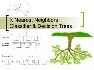
Nearest Neighbors • k-nearest neighbors • k = parameter, chosen by analyst • For a given test instance, use the k “closest” points (nearest neighbors) for performing classification • “closest” points: defined by some proximity metric, such as Euclidean Distance

Algorithm • Can’t have a CS class without pseudocode!

Requires three things • The set of stored records • Distance Metric to compute distance between records • The value of k, the number of nearest neighbors to retrieve • To classify an unknown record: • Compute distance to other training records • Identify k nearest neighbors • Use class labels of nearest neighbors to determine the class label of unknown record (e.g., by taking majority vote)

Definition of Nearest Neighbor • The k-nearest neighbors of a given example x are the k points that are closest to x. • Classification changes depending on the chosen k • Majority Voting • Tie Scenario: • Randomly choose classification? • For binary problems, usually an odd k is used to avoid ties.

Voronoi Tessellations and Decision Boundaries • When k-NN is searching for the nearest neighbor, it is partitioning the abstract feature space into a Voronoi tessellation • Each region belongs to an instance • Contains all the points in the space whose distance to that instance is less than the distance to any other instance

Decision Boundary: the boundary between regions of the feature space in which different target levels will be predicted. • Generate the decision boundary by aggregating the neighboring regions that make the same prediction.

One of the great things about nearest neighbor algorithms is that we can add in new data to update the model very easily.

What’s up with the top-right instance? • Is it noise? • The decision boundary is likely not ideal because of id13. • k-NN is a set of local models, each defined by a single instance • Sensitive to noise! • How to mitigate noise? • Choose a higher value of k.

Different Values of k Which is the ideal value of k? • Setting k to a high value is riskier with an imbalanced dataset. • Majority target level begins to dominate the feature space. k=5 k=15 k=1 k=3 Ideal decision boundary Choose k by running evaluation experiments on a training or validation set.

Choosing the right k • If k is too small, sensitive to noise points in the training data • Susceptible to overfitting • If k is too large, neighborhood may include points from other classes • Susceptible to misclassification

Computational Issues? • Computation can be costly if the number of training examples is large. • Efficient indexing techniques are available to reduce the amount of computations needed when finding the nearest neighbors of a test example • Sorting training instances?

Majority Voting • Every neighbor has the same impact on the classification: • Distance-weighted: • Far away neighbors have a weaker impact on the classification.

Scaling Issues • Attributes may have to be scaled to prevent distance measures from being dominated by one of the attributes • Example, with three dimensions: • height of a person may vary from 1.5m to 1.8m • weight of a person may vary from 90lb to 300lb • income of a person may vary from $10K to $1M Income will dominate if these variables aren’t standardized.

Standardization • Treat all features “equally” so that one feature doesn’t dominate the others • Common treatment to all variables: • Standardize each variable: • Mean = 0 • Standard Deviation = 1 • Normalize each variable: • Max = 1 • Min = 0

Query / test instance to classify: • Salary = 56000 • Age = 35

Final Thoughts on Nearest Neighbors • Nearest-neighbors classification is part of a more general technique called instance-based learning • Use specific instances for prediction, rather than a model • Nearest-neighbors is a lazy learner • Performing the classification can be relatively computationally expensive • No model is learned up-front

Classifier Comparison Eager Learners Lazy Learners • Decision Trees, SVMs • Model Building: potentially slow • Classifying Test Instance: fast • Nearest Neighbors • Model Building:fast (because there is none!) • Classifying Test Instance: slow

Classifier Comparison Eager Learners Lazy Learners • Decision Trees, SVMs • finding a global model that fits the entire input space • Nearest Neighbors • classification decisions are made locally (small k values), and are more susceptible to noise

Footnotes • In many cases, the initial dataset is not needed once similarities and dissimilarities have been computed • “transforming the data into a similarity space”

References • Fundamentals of Machine Learning for Predictive Data Analytics, 1st Edition, Kelleher et al. • Data Science from Scratch, 1st Edition, Grus • Data Mining and Business Analytics in R, 1st edition, Ledolter • An Introduction to Statistical Learning, 1st edition, James et al. • Discovering Knowledge in Data, 2nd edition, Larose et al. • Introduction to Data Mining, 1st edition, Tam et al.

Nearest Neighbors