Chi-Square as a Statistical Test
Chi-Square as a Statistical Test. Chi-square test: an inferential statistics technique designed to test for significant relationships between two variables organized in a bivariate table.

Chi-Square as a Statistical Test
E N D
Presentation Transcript
Chi-Square as a Statistical Test • Chi-square test: an inferential statistics technique designed to test for significant relationships between two variables organized in a bivariate table. • Chi-square requires no assumptions about the shape of the population distribution from which a sample is drawn.
The Chi Square Test • A statistical method used to determine goodness of fit • Goodness of fit refers to how close the observed data are to those predicted from a hypothesis • Note: • The chi square test does not prove that a hypothesis is correct • It evaluates to what extent the data and the hypothesis have a good fit
Limitations of the Chi-Square Test • The chi-square test does not give us much information about the strength of the relationship or its substantive significance in the population. • The chi-square test is sensitive to sample size. The size of the calculated chi-square is directly proportional to the size of the sample, independent of the strength of the relationship between the variables. • The chi-square test is also sensitive to small expected frequencies in one or more of the cells in the table.
Statistical Independence • Independence (statistical): the absenceofassociation between two cross-tabulated variables. The percentage distributions of the dependent variable within each category of the independent variable are identical.
Hypothesis Testing with Chi-Square Chi-square follows five steps: • Making assumptions (random sampling) • Stating the research and null hypotheses • Selecting the sampling distribution and specifying the test statistic • Computing the test statistic • Making a decision and interpreting the results
The Assumptions • The chi-square test requires no assumptions about the shape of the population distribution from which the sample was drawn. • However, like all inferential techniques it assumes random sampling.
Stating Research and Null Hypotheses • The researchhypothesis (H1) proposes that the two variables are related in the population. • The null hypothesis (H0) states that no association exists between the two cross-tabulated variables in the population, and therefore the variables are statistically independent.
H1: The two variables are related in the population. Gender and fear of walking alone at night are statistically dependent. Afraid Men Women Total No 83.3% 57.2% 71.1% Yes 16.7% 42.8% 28.9% Total 100% 100% 100%
H0: There is no association between the two variables. Gender and fear of walking alone at night are statistically independent. Afraid Men Women Total No 71.1% 71.1% 71.1% Yes 28.9% 28.9% 28.9% Total 100% 100% 100%
The Concept of Expected Frequencies Expected frequencies fe :the cell frequencies that would be expected in a bivariate table if the two tables were statistically independent. Observed frequencies fo: the cell frequencies actuallyobserved in a bivariate table.
Calculating Expected Frequencies fe = (column marginal)(row marginal) N To obtain the expected frequencies for any cell in any cross-tabulation in which the two variables are assumed independent, multiply the row and column totals for that cell and divide the product by the total number of cases in the table.
Chi-Square (obtained) • The test statistic that summarizes the differences between the observed (fo) and the expected (fe) frequencies in a bivariate table.
Calculating the Obtained Chi-Square fe= expected frequencies fo = observed frequencies
The Sampling Distribution of Chi-Square • The sampling distribution of chi-square tells the probability of getting values of chi-square, assumingno relationship exists in the population. • The chi-square sampling distributions depend on the degrees of freedom. • The sampling distribution is not one distribution, but is a family of distributions.
The Sampling Distribution of Chi-Square • The distributions are positively skewed. The research hypothesis for the chi-square is always a one-tailed test. • Chi-square values are always positive. The minimum possible value is zero, with no upper limit to its maximum value. • As the number of degrees of freedom increases, the distribution becomes more symmetrical.
Determining the Degrees of Freedom df = (r – 1)(c – 1) where r = the number of rows c = the number of columns
Calculating Degrees of Freedom How many degrees of freedom would a table with 3 rows and 2 columns have? (3 – 1)(2 – 1) = 2 2 degrees of freedom
The Chi Square Test (we will cover this in lab;) • The general formula is (O – E)2 c2 =S E • where • O = observed data in each category • E = observed data in each category based on the experimenter’s hypothesis • S = Sum of the calculations for each category
Gene affecting wing shape • c+ = Normal wing • c = Curved wing • Gene affecting body color • e+ = Normal (gray) • e = ebony • Consider the following example in Drosophila melanogaster • Note: • The wild-type allele is designated with a + sign • Recessive mutant alleles are designated with lowercase letters • The Cross: • A cross is made between two true-breeding flies (c+c+e+e+ and ccee). The flies of the F1 generation are then allowed to mate with each other to produce an F2 generation.
The outcome • F1 generation • All offspring have straight wings and gray bodies • F2 generation • 193 straight wings, gray bodies • 69 straight wings, ebony bodies • 64 curved wings, gray bodies • 26 curved wings, ebony bodies • 352 total flies • Applying the chi square test • Step 1: Propose a null hypothesis (Ho) that allows us to calculate the expected values based on Mendel’s laws • The two traits are independently assorting
Step 2: Calculate the expected values of the four phenotypes, based on the hypothesis • According to our hypothesis, there should be a 9:3:3:1 ratio on the F2 generation
(O1 – E1)2 (O2 – E2)2 (O3 – E3)2 (O4 – E4)2 E1 E2 E3 E4 (193 – 198)2 (69 – 66)2 (64 – 66)2 (26 – 22)2 66 66 22 198 • Step 3: Apply the chi square formula c2 = + + + c2 = + + + c2 = 0.13 + 0.14 + 0.06 + 0.73 c2 = 1.06
Step 4: Interpret the chi square value • The calculated chi square value can be used to obtain probabilities, or P values, from a chi square table • These probabilities allow us to determine the likelihood that the observed deviations are due to random chance alone • Low chi square values indicate a high probability that the observed deviations could be due to random chance alone • High chi square values indicate a low probability that the observed deviations are due to random chance alone • If the chi square value results in a probability that is less than 0.05 (ie: less than 5%) it is considered statistically significant • The hypothesis is rejected
Step 4: Interpret the chi square value • Before we can use the chi square table, we have to determine the degrees of freedom (df) • The df is a measure of the number of categories that are independent of each other • If you know the 3 of the 4 categories you can deduce the 4th (total number of progeny – categories 1-3) • df = n – 1 • where n = total number of categories • In our experiment, there are four phenotypes/categories • Therefore, df = 4 – 1 = 3 • Refer to Table 2.1
Step 4: Interpret the chi square value • With df = 3, the chi square value of 1.06 is slightly greater than 1.005 (which corresponds to P-value = 0.80) • P-value = 0.80 means that Chi-square values equal to or greater than 1.005 are expected to occur 80% of the time due to random chance alone; that is, when the null hypothesis is true. • Therefore, it is quite probable that the deviations between the observed and expected values in this experiment can be explained by random sampling error and the null hypothesis is not rejected. What was the null hypothesis?