Chi-Square Test
Chi-Square Test. Mon, Apr 19 th , 2004. Chi-Square ( 2 ). Are 2 categorical variables related (correlated) or independent of each other? Compares # in categories that would be expected by chance (E) to # in categories actually observed (O)


Chi-Square Test
E N D
Presentation Transcript
Chi-Square Test Mon, Apr 19th, 2004
Chi-Square (2) • Are 2 categorical variables related (correlated) or independent of each other? • Compares # in categories that would be expected by chance (E) to # in categories actually observed (O) • Null hyp (Ho) – no relationship between 2 variables (they’re independent of ea.other) • Alternate (Ha) – the 2 variables are related (not independent)
2 Formula • 2 = [(fo – fe)2] fe So we’ll compare observed and expected frequencies for each cell in the table…
Is age (<30 v. >30) related to preference for analog/digital watches? Example
Step 1: Compute Marginals Marginals are the row and column totals: 140 60 100 20 80
Step 2: Compute Expected Frequencies (fE) • fE = (Column marginal * Row marginal ) / N For people under 30: fe (digital) = 100 * 140 / 200 = 70 fe (analog) = 80*140 / 200 = 56 fe (undec) = 20*140 / 200 = 14 Over 30: fe (digital) = 100*60 / 200 = 30 fe (analog) = 80*60 / 200 = 24 fe (undec) = 20*60 / 200 = 6
Step 3: Compute X2 • Find difference (residual) betw observed & expected for each cell (fo – fe) • Square those differences • Divide squared differences by fe • Sum the results
(cont.) • Last step: Add up (fo-fe)2 / fe • 2 = 5.71 + 4.57 + 1.14 + 13.33 + 10.67 + 2.67 = 38.09 • Step 4: Compare to 2 critical with df = (# columns – 1) (# rows – 1) • Here df = (2-1)(3-1) = 2 df, = .05, critical = 5.99
Hypothesis Test • If 2 observed > 2 critical, reject Ho • Reject Ho conclude there is a relationship between the 2 variables • Here, 38.09 > 5.99, reject Ho, there is a relationship between age & watch preference
In SPSS • Analyze Descriptive Stats Crosstabs • Choose whichever variable you’d like for ‘row variable’ and the other for ‘column variable’ • Click “Statistics” button, and check chi-squared option • Click “Cells” Button, choose “expected count”
SPSS (cont.) • Output – look for “Pearson chi-sq” and “Asymp Sig” column gives significance value for chi-sq test: • If “Asymp Sig” value is < .05 (alpha), reject Ho • Note there is an option for clustered graphing, read this example in the lab