The Chi-Square Test
The Chi-Square Test. E. Çiğdem Kaspar,Ph.D. Assist. Prof. Yeditepe University, Faculty of Medicine Biostatistics. The Chi-Square Test. OBSERVED AND THEORETICAL FREQUENCIES


The Chi-Square Test
E N D
Presentation Transcript
The Chi-Square Test E. Çiğdem Kaspar,Ph.D. Assist. Prof. Yeditepe University, Faculty of Medicine Biostatistics
The Chi-Square Test OBSERVED AND THEORETICAL FREQUENCIES As we have already seen many times, results obtained in samples do not always agree exactly with theoretical results expected according to rules of probability. For example, although theoretical considerations lead us to expect 50 heads and 50 tails when we toss a fair coin 100 times, it is rare that these results are obtained exactly.
The Chi-Square Test Suppose that in a particular sample a set of possible events E1,E2,E3,….,Ek (see fallowing Table ) are observed to occur with frequencies o1,o2,o3,….,ok, called observed frequencies, and that according to probability rules they are expected to occur with frequencies e1,e2,e3,…..,ek, called expected or theoretical frequencies.
The Chi-Square Test Often we wish to know whether observed frequencies differ significantly from expected frequencies. For the case where only two events E1 and E2 are possible (sometimes called a dichotomy or dichotomous classification), as for example heads or tails, defective or non-defective bolts, etc.,
The Chi-Square Test DEFINITION OF 2 A measure of the discrepancy existing between observed and expected frequencies is supplied by the statistic 2 (read chi-square) given by
The Chi-Square Test where if the total frequency is N, An expression equivalent to (1) is
The Chi-Square Test If 2=0, observed and theoretical frequencies agree exactly, while if 2 > 0, they do not agree exactly. The larger the value of 2, the greater is the discrepancy between observed and expected frequencies. The sampling distribution of 2 is approximated very closely by the chi-square distribution if expected frequencies are at least equal to 5, the approximation improving for larger values.
The Chi-Square Test The number of degrees of freedom v is given by (a) v = k — 1 if expected frequencies can be computed without having to estimate population parameters from sample statistics. Note that we subtract 1 from k because of the constraint condition (2) which states that if we know k — 1 of the expected frequencies the remaining frequency can be determined. (b) v = k — 1 — m if the expected frequencies can be computed only by estimating m population parameters from sample statistics.
The Chi-Square Test SIGNIFICANCE TESTS In practice, expected frequencies are computed on the basis of a hypothesis H0. If under this hypothesis the computed value of 2 given by (1) or (3) is greater than some critical value (such as 20.95 or 20.99, which are the critical values at the 0.05 and 0.01 significance levels respectively), we would conclude that observed frequencies differ significantly from expected frequencies and would reject H0 at the corresponding level of significance. Otherwise we would accept it or at least not reject it. This procedure is called the chi-square test of hypothesis or significance.
The Chi-Square Test It should be noted that we must look with suspicion upon circumstances where 2 is too close to zero since it is rare that observed frequencies agree too well with expected frequencies. To examine such situations, can determine whether the computed value of 2 is less than 20.05 or 20.01 in which cases we would decide that the agreement is too good at the 0.05 or 0.01 levels of significance respectively.
The Chi-Square Test THE CHI-SQUARE TEST FOR GOODNESS OF FIT The chi-square test can be used to determine how well theoretical distributions, such as the normal, binomial, etc., fit empirical distributions, i.e. those obtained from sample data.
The Chi-Square Test CONTINGENCY TABLES Table above, in which observed frequencies occupy a single row, is called a one-way classification table. Since the number of columns is k, this is also called a 1 x k (read "1 by k") table. By extending these ideas we can arrive at two-way classification tables or h + k tables in which the observed frequencies occupy h rows and k columns. Such tables are often called contingency tables.
The Chi-Square Test Corresponding to each observed frequency in an h x k contingency table, there is an expected or theoretical frequency which is computed subject to some hypothesis according to rules of probability. These frequencies which occupy the cells of a contingency table are called cell frequencies. The total frequency in each row or each column is called the marginal frequency.
The Chi-Square Test To investigate agreement between observed and expected frequencies, we compute the statistic Where the sum is taken over all cells in the contingency table, the symbols oj and ej representing respectively the observed and expected frequencies in the j th cell. This sum which is analogous to (1) contains hk terms. The sum of all observed frequencies is denoted by N and is equal to the sum of all expected frequencies (compare with equation (2)).
The Chi-Square Test As before, the statistic (5) has a sampling distribution given very closely by (4), provided expected frequencies are not too small. The number of degrees of freedom v of this chi-square distribution is given for h > 1, k > 1 by (a) v = (h — 1)(k — 1) if the expected frequencies can be computed without having to estimate population parameters from sample statistics.
The Chi-Square Test (b) v = (h — 1)(k — 1) — m if the expected frequencies can be computed only by estimating m population parameters from sample statistics. Significance tests for h x k tables are similar to those for 1 x k tables. Expected frequencies are found subject to a particular hypothesis Ho. A hypothesis commonly assumed is that the two classifications are independent of each other. Contingency tables can be extended to higher dimensions. Thus, for example, we can have h x k X I tables where 3 classifications are present.
The Chi-Square Test YATES' CORRECTION FOR CONTINUITY When results for continuous distributions are applied to discrete data, certain corrections for continuity can be made as we have seen in previous chapters. A similar correction is available when the chi-square distribution is used. The correction consists in rewriting (1) as and is often referred to as Yates' correction. An analogous modification of (5) also exists.
The Chi-Square Test SIMPLE FORMULAE FOR COMPUTING 2 Simple formulae for computing 2 which involve only the observed frequencies can be derived. In the following we give the results for 2 x 2 and 2x3 contingency tables. 2x2 Tables
The Chi-Square Test With Yates' correction this becomes 2x3 Tables
The Chi-Square Test where we have used the general result valid for all contingency tables, The result (9) for 2 x k tables where k > 3, can be generalized.
The Chi-Square Test Fisher’s an analysis of precision Chi-square a1 or b1 or c1 or d1 < 5 P=(S1! x S2 ! x S3 ! x S4 !)/(T ! x a ! x b ! x c ! x d !)
The Chi-Square Test P = (42! x 58! x 11! x 89! ) / ( 100! x 3! x 8! x 39! x 50! ) + (42! x 58! x 11! x 89! ) / ( 100! x 2! x 9! x 40! x 49! ) + (42! x 58! x 11! x 89! ) / ( 100! x 1! x 10! x 41! x 48! ) + (42! x 58! x 11! x 89! ) / ( 100! x 0! x 11! x 42! x 47! ) P = 0.027 Result : The differencies of ditribution is significant
The Chi-Square Test COEFFICIENT OF CONTINGENCY A measure of the degree of relationship, association or dependence of the classifications in a contingency table is given by which is called the coefficient of contingency. The larger the value of C, the greater is the degree of association. The number of rows and columns in the contingency table determines the maximum value of C, which is never greater than one. If the number of rows and columns of a contingency table is equal to k, the maximum value of C is given by ((k -1)/k)(1/2).
The Chi-Square Test CORRELATION OF ATTRIBUTES Because classifications in a contingency table often describe characteristics of individuals or objects, they are often referred to as attributes and the degree of dependence, association or relationship is called correlation of attributes. For k x k tables we define as the correlation coefficient between attributes or classifications. This coefficient lies between 0 and 1 . For 2x2 tables in which k = 2, the correlation is often called tetrachoric correlation.