Design of Tree Algorithm

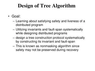
1. Design of Tree Algorithm • Goal: • Learning about satisfying safety and liveness of a distributed program • Utilizing invariants and fault-span systematically while designing distributed programs • design a tree construction protocol systematically by constructing its invariant and fault-span • This is known as nonmasking algorithm since safety may not be preserved during recovery

2. Intuition in Design of the Program • Invariant • Set of constraints that should be true in the absence of faults • Alternatively, after recovery is complete • Fault-span • Set of constraints that should be true even in the presence of faults • One safety property of interest • Constraints in fault-span should be preserved • One liveness property of interest • Constraints in the invariant should be eventually satisfied

3. Ideal State • Given is a graph G = (V, N). • V denotes the set of processes/nodes • N denotes edges that show adjacency of processes • Each process j maintains a variable P.j. P.j denotes the parent of j in the tree. • Each process also has a unique ID • In an ideal state the graph imposed by the parent relation forms a tree • This will be one constraint in the invariant • What are the program actions inside the invariant?

4. Faults • Can fail or repair a process • Goal: Reconstruct the tree with the available processes

5. Due to faults, we may have • Unrooted trees • Because some node’s parent has failed • Multiple (rooted) trees • For example, when a node is repaired, it may form a tree by itself • Observe that there are no cycles. In other words, in the presence of faults, a cycle is not created. • We may want to preserve this during reconstruction. • I.e., this constraint should be in the fault-span

6. Predicates for Fault-Span (1) • The graph imposed by the parent relation is a forest

7. Approach for Reconstruction • Dealing with unrooted trees • Somehow the nodes in unrooted trees should be informed so that they know that they are in an unrooted tree • Approach: Introduce a variable color (col) • Green = node thinks it is in rooted tree • Red = node thinks it is in unrooted tree

8. What would I like to be true about colors in invariant? • Ok with gg, rr, • If j and parent of j are alive then • j is red  parent of j is red • What would I like to be true about colors in fault span? • Ok with gg, rr, rg • If node j is red => parent of j is red or parent of j has failed

9. Difference between fault span and invariant • States where j is green and parent of j is either red or parent of j has failed • State that is in fault span but not invariant • Provide recovery from here to invariant

10. Predicate in Invariant • What property would have to be satisfied to obtain the meaning of the colors? • S1 = (P.j  N.j  col.(P.j) = red)  col.j = red • Suppose this is not true, how to fix it?

11. Action (1) col.j = green (P.j  N.j  col.(P.j) = red)  col.j = red

12. Variant Function • Will the previous action, result in a state where S1 will be true for all nodes? • Need to identify a variant function • Property of the variant function • Its value never increases • Execution of this action decreases the value • The value is bounded from below • The function is well-founded

13. Variant function

14. Predicate in Fault-Span (2) • The graph imposed by the parent relation is a forest  • col.j = red  (P.j  N.j  col.(P.j) = red) • Recall that we need to check if program actions will preserve this predicate!

15. Note • Observe that Action (1) is aimed at correcting a predicate in the invariant • Must ensure that during correction, the fault-span constraints are not violated

16. Predicate in Invariant • (P.j  N.j  col.(P.j) = red)  col.j = red • col.j = green

17. Action (2) • When should a node set its color to green • Need to ensure that constraints of fault-span are not violated • Need to ensure that constraints of previous predicates in invariant are not violated

18. Action (2) col.j = red  (????)  col.j = green Choose ???? so that this action does not affect fault-span predicate/previous predicates in invariant

19. Action (2) col.j = red  (j is a leaf)  col.j = green, P.j = j

20. After fixing S1 and S2 • All nodes are green • Only way to satisfy constraint S1 is to ensure that P.j is a neighbor of j

21. Merging Multiple Trees • Introduce variable root • root.j denotes the ID of the process that j believes to be the root • If a process finds another process with higher root value, it can choose to switch to it.

22. Action (2) modified col.j = red  (j has no children)  col.j = green, P.j = j, root.j = j

23. Predicate in Invariant (3) • (P.j  N.j  col.(P.j) = red)  col.j = red • col.j = green • root.j = root.k

24. Action (3) root.j < root.k  (????)  root.j = root.k, P.j = k

25. Action (3) root.j < root.k  col.j = green /\ col.k = green  root.j = root.k, P.j = k

26. Predicate in Fault-Span • The graph imposed by the parent relation is a forest  • col.j = red  (P.j  N.j  col.(P.j) = red) • col.(P.j) = green  root.j root.(P.j) • j  root.j • j = root j iff j = P.j

27. Recovery Action for Process Recovery of node j  col.j = red, P.j = j, root.j = j

28. Observations: Stepping Back • We encountered some problems in design of this protocol • Consider the action that changed its color to green • If allowed to execute as is the fault span predicate would have been violated • We fixed it by restricting when the action can be executed • Consider the action by which j changes tree to k • There was a potential to cause a cycle • We fixed it by strengthening (reducing) the fault span so that such a state is not reached in the presence of faults • Another possible choice was to weaken (expand) fault span so that the state where j changes tree to form cycle is included in it. • We will see example of this in next module

29. Observations (continued) • For the case where we considered where j changes tree to k • We could have argued that such a state could not exist. • But that would require one to consider sequences of program executions. • Generally, humans are not very good at this: • The use of invariant/fault span allowed us to only consider one action at a time. • This is typically a lot easier than being able to analyze all possible sequences. • Variant functions play a similar role for liveness.

30. Analyzing Sequences • Consider the following code where there are two threads and executes the code below For (int j = 0 ; j < 5 ; j++) temp = sum ; sum = temp + 1 • Sum is a shared variable initialized to 0. And, j and temp are private variables of each thread. • What is the final value of sum

31. Assumptions Made in the Protocol • If a node fails then its neighbors can detect it • Detection is accurate, i.e. a live node would not be suspected and a failed node is guaranteed to be suspected. • Is this assumption necessary? • What would we do if we did not have such an assumption? • Can we still re-build the tree? • We will study this aspect a little later.