Analysis of Covariance

Analysis of Covariance

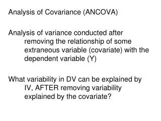
ANOVA is a class of statistics developed to evaluate controlled experiments. Experimental control, random selection of subjects, and random assignment of subjects to subgroups are devices to control or hold constant all the other (UNMEASURED) influences on the dependent (Yij) variable so that the effects of the independent (Xij) variable can be assessed. Without experimental control, random selection, and random assignment, other (non-random) differences besides the treatment variable enter the picture.Remember: Inferential statistics only assess the likelihood that chance could have affected the sample results; they do not take into account non-random factors.

For example, without randomly selecting students and compelling them to take PPD 404, then randomly assigning them to an instructor, plus controlling their lives for an entire semester (e.g., forbidding them to work), differences that are not random creep in.To some extent, this problem of uncontrolled, non-random differences can be compensated for by introducing covariates as statistical controls. Covariates are continuous variablesthat hold constant non-random differences. For example, by asking students how many hours per week they were working, we could add this variable to our ANOVA model. Let's look briefly at the analysis of covariance with one of the classic examples in the statistical literature.

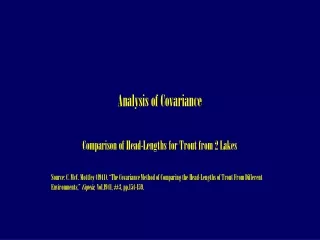
The data are from an experiment involving the use of two drugs for treating leprosy. Drug A and Drug B were experimental drugs; Drug C was a placebo. Subjects were children in the Philippines suffering from leprosy. Thirty children who were taken to a clinic were given either Drug A, B, or C (the treatments) in order of their arrival. Thus each subgroup consisted of 10 children. The outcome measure, Yij, was a microscopic count of leprosy bacilli in samples taken from six body sites on each child at the end of the experiment. Data are in the following table.

——————————————————————————————————————————————————————— Group A Group B Group CY Y2 X X2 XY Y Y2 X X2 XY Y Y2 X X2 XY——————————————————————————————————————————————————————— 6 36 11 121 66 0 0 6 36 0 13 169 16 256 208 0 0 8 64 0 2 4 6 36 12 10 100 13 169 130 2 4 5 25 10 3 9 7 49 21 18 324 11 121 198 8 64 14 196 112 1 1 8 64 8 5 25 9 81 4511 121 19 361 209 18 324 18 324 324 23 529 21 441 483 4 16 6 36 24 4 16 8 64 32 12 144 16 256 19213 169 10 100 130 14 196 19 361 266 5 25 12 144 60 1 1 6 36 6 9 81 8 64 72 16 256 12 144 192 8 64 11 121 88 1 1 5 25 5 1 1 7 49 7 0 0 3 9 0 9 81 15 225 135 20 400 12 144 240——————————————————————————————————————————————————————— 53 475 93 1069 645 61 713 100 1248 875 123 1973 129 1805 17555.3 9.3 6.1 10.0 12.3 12.9n1 = 10 n2 = 10 n3 = 10Y = 237 X = 322 N = 30_ _Y = 7.90 X = 10.73

First, let’s perform a one-way analysis of variance on these data. As a short-cut for calculating the sum of squares, we will use the following algorithm:SS = Y2 - (Y)2 / NThis is read: sum of squares equals the sum of the squared values of Y minus the sum of the Y-values squared with the difference between them divided by N. This short-cut was developed to speed up calculations in the days before widespread use of computer software.Three variations of this short-cut will be used.

First, let's find the totalsum of squares. This is the sum of all the squared Y-values less the sum of the Y-values squared with the difference between them divided by N:SSTotal(Y) = (475 + 713 + 1973) - [(237)2/30]SSTotal(Y) = (3161) - (56169/30)SSTotal(Y) = 3161 - 1872SSTotal(Y) = 1289

Next, the betweensum of squares can be obtained by applying the short-cut equation: SSBetween(Y) = [(53)2/10 + (61)2/10 + (123)2/10] - [(237)2/30]SSBetween(Y) = 2166 - 1872SSBetween(Y) = 294

Finally, the sum of squares within:SSWithin(Y) = SSTotal(Y) - SSBetween(Y)SSWithin(Y) = 1289 - 294SSWithin(Y) = 995Degrees of freedom are as before: N - 1 for total, J - 1 for between, and N - J for within.

These results can be assembled in the usual ANOVA summary table.——————————————————————————————————————————————————————————————Source SS df Mean Square F——————————————————————————————————————————————————————————————Between 294 2 147.000 3.989GroupsWithin 995 27 36.852GroupsTotal 1289 29——————————————————————————————————————————————————————————————

Because we do not want to "jump to conclusions" with the experimental drugs, an alpha level of 0.05 is too modest. Let's set alpha at 0.01. This means that we have only one chance in 100 of wrongly rejecting the null hypothesis (ruling out chance as the explanation for differences in the effectiveness of the drugs). With alpha = 0.01, the critical value of F with 2 and 27degrees of freedom is 5.49 (Appendix 3, p. 545). Since F is only 3.989, we CANNOT reject the null hypothesis. There is no evidence that either Drug A or Drug B is different from the placebo, Drug C, nor is there evidence that Drugs A and B differ from one another.

The researchers wanted to be sure that the children in each of the three groups were equally ill at the beginning of the experiment. Perhaps one of the drugs was effective, but, because the children who received it were more sick than those in the other groups, its effects were masked. A measure of illness at the START of the experiment was added to the statistical analysis as a control variable—as a covariate. This covariate was the count of bacilli at the same six body sites, but these counts were taken BEFORE any drugs were given. These data are in the table under columns headed X.

The general linear model that includes the influence of this covariate is written:Yij =  + jX1ij + X2ij + ijwhere is a linear coefficient expressing the influence of the covariate, X2ij, on the dependent variable, Yij. If the covariate has no influence,  = 0.0. Therefore, the X2ij products all would be 0.0, and this term would drop out, leaving Yij =  + jX1ij + ij

To adjust for the presence of the covariate, we need to calculate sums of squares and degrees of freedom for the covariate, X2, AS WELL AS for the covariance between X2 and Y. We construct covariance sums of squares from the cross-products, XY (the final column in each of the three table panels). Total sum of squares, between sum of squares, and within sum of squares for the covariate, X2, are straightforward. For the totalsum of squares for X:SSTotal(X) = (1069 + 1248 + 1805) - [(322)2/30]SSTotal(Y) = (4122) - (103,684/30)SSTotal(X) = 4122 - 3456SSTotal(X) = 666

For the betweensum of squares:SSBetween(X) = [(93)2/10 + (100)2/10 + (129)2/10] - [(322)2/30]SSBetween(X) = 3529 – 3456SSBetween(X) = 73And for the withinsum of squares:SSWithin(X) = SSTotal(X) - SSBetween(X)SSWithin(X) = 666 – 73SSWithin(X) = 593

For the cross-products, we use the same approach; e.g., for the cross-product totalsum of squares:SSTotal(XY) = (645 + 875 + 1755) - [(322)(237)/30]SSTotal(XY) = (3277) - (76,314/30)SSTotal(XY) = 3277 – 2544SSTotal(XY) = 733

For the cross-product between sum of squares:SSBetween(XY) = [(53)(93)10 + (61)(100)10 + (123)(129)/10] - [(322)(237)/30]SSBetween(XY) = 2690 - 2544SSBetween(YX) = 146And for the cross-product within sum of squares:SSWithin(XY) = SSTotal(XY) - SSBetween(XY)SSWithin(XY) = 733 - 146SSWithin(XY) = 587

Adjustments to the simple ANOVA results for the presence of the covariate should also look familiar. We need to adjust the within sum of squares, the between sum of squares, the within degrees of freedom, and the between degrees of freedom. Total sum of squares and total degrees of freedom are unchanged because (a) we are still trying to account for total variance in the dependent variable, Yij, and (b) we have the same number of subjects, 30.

The withinsum of squares adjustment is:SSWithin(Adj) = SSWithin(Y) - [(SSWithin(XY))2 / SSWithin(X)]SSWithin(Adj) = 995 - [(587)2 / 593]SSWithin(Adj) = 995 - (344,569 / 593)SSWithin(Adj) = 995 – 581SSWithin(Adj) = 414

The adjustment for the betweensum of squaresis:SSBetween(Adj) = SSTotal - SSWithin(Adj)SSBetween(Adj) = 1298 - 414SSBetween(Adj) = 875We lose a degree of freedom within from the total degrees of freedom for the presence of the covariate. The adjustment isdfWithin(Adj) = N - J - Kwhere K is the number of covariates. Here,dfWithin(Adj) = 30 - 3 - 1 = 26

Because of the IDENTITY between degrees of freedom, the adjustment for the betweendegrees of freedom is simplydfBetween(Adj) = dfTotal - dfWithin(Adj)dfBetween(Adj) = 29 - 26 = 3The analysis of covariance results are contained in following table.

——————————————————————————————————————————————————————————————Source SS df Mean Square F——————————————————————————————————————————————————————————————Between 875 3 291.667 18.317GroupsWithin 414 26 15.923GroupsTotal 1289 29——————————————————————————————————————————————————————————————The presence of the covariate in the general linear model makes quite a difference. The within sum of squares has been reduced to 414 from 995 with the loss of only one degree of freedom. The between sum of squares—reflecting the differences among drugs—has nearly tripled, from 294 to 875 with a gain of only one degree of freedom. As a result, the F-ratio is now 18.317.

With alpha at 0.01 and 3 and 26 degrees of freedom, the critical valueis now 4.64 (Appendix 3, p. 545). Thus, we REJECT the null hypothesis that none of the three drugs was different from any other:H0: 1 = 2 = 3We conclude that the effect of at least ONE of the drugs differed from that of the others when we control for the seriousness of illness at the start of the experiment. To determine which drug(s) differ, we need to perform a comparison test such as the Scheffé test.

First, we need to "adjust" the subgroup means for the effect of the covariate. To do this, we need to calculate the value of the constant, . With this value we can calculate adjusted subgroup means. The algorithm is: = SSWithin(XY) / SSWithin(X)From the analysis of variance summary table, = (587) / (593) = 0.990The adjustment for the covariate is:

The adjustments for the influence of the covariate are: _Yadj = 5.3 - [0.99(9.3 - 10.73)] = 6.72 _ Yadj = 6.1 - [0.99(10.0 - 10.73)] = 6.82 _ Yadj = 12.3 - [0.99(12.9 - 10.73)] = 10.15We can test the significance of difference between pairs of these subgroup means using the post hoc comparison method described earlier. Visual inspection of these adjusted means shows that children receiving Drug A and Drug B had fewer leprosy bacilli at the end of the experiment than did those children receiving Drug C, the placebo, controlling for pre-treatment illness.

Using SAS for Analysis of Variance and CovarianceLIBNAME perm 'a:\';LIBNAME library 'a:\';OPTIONS NODATE NONUMBER PS=66;PROC GLM DATA=perm.drugtest;CLASS drug;MODEL posttest = drug;TITLE1 'One‑Way Analysis of Variance Example';TITLE2;TITLE3 'PPD 404';RUN;PROC GLM DATA=perm.drugtest;CLASS drug;MODEL posttest = drugpretest;TITLE1 'Analysis of Covariance Example';TITLE2;TITLE3 'PPD 404';RUN;

One‑Way Analysis of Variance Example PPD 404 General Linear Models Procedure Class Level InformationClass Levels ValuesDRUG 3 A B C Number of observations in data set = 30 General Linear Models ProcedureDependent Variable:POSTTESTSum of MeanSource DF Squares Square F Value Pr > FModel 2 293.6000000 146.8000000 3.980.0305Error 27 995.1000000 36.8555556Corrected Total 29 1288.7000000R‑Square C.V. Root MSE Y Mean0.227826 76.84655 6.070878 7.90000000Source DF Type I SS Mean Square F Value Pr > FDRUG 2 293.6000000 146.8000000 3.98 0.0305Source DF Type III SS Mean Square F Value Pr > FDRUG 2 293.6000000 146.8000000 3.98 0.0305

Analysis of Covariance Example PPD 404 General Linear Models Procedure Class Level Information Class Levels Values DRUG 3 A B C Number of observations in data set = 30Dependent Variable: POSTTEST Sum of MeanSource DF Squares Square F Value Pr > FModel 3 871.4974030 290.4991343 18.10 0.0001Error 26 417.2025970 16.0462537Corrected Total 29 1288.7000000R‑Square C.V. Root MSE Y Mean0.676261 50.70604 4.005778 7.90000000Source DF Type I SS Mean Square F Value Pr > FDRUG 2 293.6000000 146.8000000 9.15 0.0010PRETEST 1 577.8974030 577.8974030 36.01 0.0001Source DF Type III SS Mean Square F Value Pr > FDRUG 2 68.5537106 34.2768553 2.14 0.1384PRETEST 1 577.8974030 577.8974030 36.01 0.0001

Analysis of Covariance