Download
1 / 13
130 likes | 255 Vues
This appendix explores the application of the binomial distribution in finance, specifically for evaluating call options. It discusses fundamental concepts such as what an option is and describes both the simple binomial option pricing model and the generalized binomial option pricing model. The appendix includes detailed examples illustrating how to calculate option values at maturity using binomial methods, equations for pricing, and scenarios involving stock price fluctuations. This resource is valuable for finance professionals and students interested in options pricing techniques.

E N D
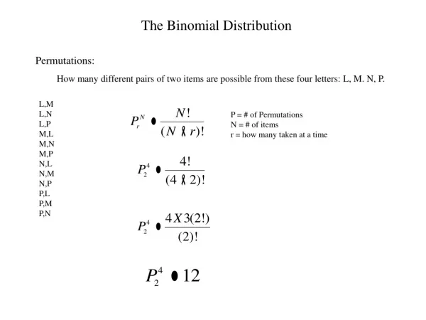
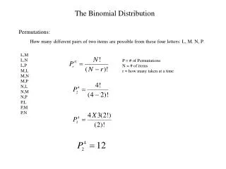
Appendix 17A Application of the Binomial Distribution to Evaluate Call Options
Appendix 17A: Applications of the Binomial Distribution to Evaluate Call Options In this appendix, we show how the binomial distribution is combined with some basic finance concepts to generate a model for determining the price of stock options. What is an option? The simple binomial option pricing model The Generalized Binomial Option Pricing Model
Appendix 17A: Applications of the Binomial Distribution to Evaluate Call Options (17A.1) (17A.2) (17A.3) (17A.4)
Appendix 17A: Applications of the Binomial Distribution to Evaluate Call Options (17A.5) (17A.6) (17A.7) (17A.8)
Appendix 17A: Applications of the Binomial Distribution to Evaluate Call Options Table 17A.1 Possible Option Value at Maturity
Appendix 17A: Applications of the Binomial Distribution to Evaluate Call Options Let X = $100 S = $100 u = (1.10). so uS = $110 d = (.90), so dS = $90 R = 1 + r = 1 + 0.07 = 1.07 Next we calculate the value of p as indicated in Equation (17A.7): Solving the binomial valuation equation as indicated in Equation (17A.8), we get C = [.85(10) + .15(0)] / 1.07 = $7.94.
Appendix 17A: Applications of the Binomial Distribution to Evaluate Call Options CT = Max [0, ST – X] (17A.9) Cu = [pCuu+ (1 – p)Cud] / R (17A.10) Cd= [pCdu+ (1 – p)Cdd] / R (17A.11) (17A.12) (17A.13)
Example 17A.1 Figure 17A.1 Price Path of Underlying Stock and Value of Call Option Source: R.J.Rendelman, Jr., and B.J.Bartter (1979), “Two-State Option Pricing,” Journal of Finance 34(December), 1906.
Example 17A.1 In addition, we can Equation (17A.13) to determine the value of the call option. The cumulative binomial density function can be defined as: (17A.14) where n is the number of periods,kis the number of successful trials,
Appendix 17A: Applications of the Binomial Distribution to Evaluate Call Options (17A.15) C1 = Max [0, (1.1)3(.90)0(100) – 100] = 33.10 C2 = Max [0, (1.1)2(.90) (100) – 100] = 8.90 C3 = Max [0, (1.1) (.90)2(100) – 100] = 0 C4 = Max [0, (1.1)0(.90)3(100) – 100] = 0
Appendix 17A: Applications of the Binomial Distribution to Evaluate Call Options
Appendix 17A: Applications of the Binomial Distribution to Evaluate Call Options (17A.16) (17A.17)
Appendix 17A: Applications of the Binomial Distribution to Evaluate Call Options