
Comprehensive Guide to Quantitative Data Analysis
E N D
Presentation Transcript
QUANTITATIVE DATA ANALYSIS Researchers convert data to numerical form and subject them to statistical analysis From ch 14. Earl Babbie, The Practice of Social Research and Lawrence Newman, Basics of Social Research, ch. 10.
Quantitative analysis is handled by computer programs like SPSS. • The task of quantification is to reduce idiosyncratic items of information to a more limited sets of attributes composing a variable. • Best to keep quantification coding based on greater detail. Code categories can be collapsed later anytime if lesser detail is needed.
Begin with a well developed coding scheme, Develop categories to reflect dimensions of the variable, i.e. various attributes composing a variable Your coding choice should match your research purpose and be intersubjective.
A codebook is a document that describes the location of variable and lists the assignments of codes to the attributes composing those variables. Data need to be converted into machine readable format, every category should get a number.
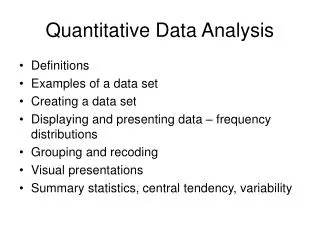
I. Univariate Analysis • Frequency Distributions • The number of times that various attributes of a variable are observed in a sample (also called marginals) • Central Tendency • Presenting data in the form of an average of a measure of central tendency.
Central Tendency Measures • Mean: dividing the sum of the values by the total number of cases. • Mode: most frequently occurring attribute. • Median: the middle attribute in a RANKED distribution of observed attributes, the 50th percentile. • These measures give the CENTER of a distribution.
Measures of Dispersion/Variation • Measures the dispersion or variability around the center • Remember the standard error of a sampling distribution, measures the dispersion around the population parameter. • Three Measures of Dispersion • 1. Range: The distance between the highest and lowest Value. • 2. Percentile: Tells you the score at a specific spot within the distribution- median is 50th percentile, 25th percentile would be the spot that has 25% below and 75% above. 95th percentile would have how many above and how many below the spot?
3. Standard Deviation: • Requires a ratio level measure to calculate. • It gives the average (mean) distance between all scores and the mean score. • It helps you make comparisons in distributions- for example a low or zero standard deviation means that all cases are very close to or identical with the mean, while a large standard deviation implies that individual scores are in general quite different to the mean
Steps in the calculation of standard deviation • First calculate the mean of the distribution • Then subtract each score from the mean • Square the result of each subtracted score from the mean, add them all together to get one number • divide that number by the number of cases to get the “Variance” • Square root of the variance is the standard deviation
Z scores are standardized scores for individual cases calculated using the mean of the distribution and its standard deviation • Z= Score- MEAN / Standard deviation • 95% of the cases lie within + or – 2 standard deviations from the mean, 68% lie within one standard deviation (+ or -) of the mean.
II.Bivariate Relationships • Univariate stats describe one variable in isolation, bivariate relationships are about two variables and whether they co-vary or are independent. • Covariation: means things go together or that they are associated. E.g. People who have high values on the income variable also have high values on the life expectancy variable. • Independence: means there is no relationship between variables E.g. if people with many brothers and sisters have the same life expectancy as those with fewer then “number of sibilings” is independent of or not related to “life expectancy.”
Three techniques initially allow you to see whether a relationship exists between two variables • 1. A scatterplot of the two variables, to see if the “scatter” forms a pattern • 2. A cross-tabulation or percentaged contingency-table. • 3. A zero-order correlation or statistical measure of association
Measures of Association: Chi-Square tells you if the relationship between the variables is statistically significant, while Lambda (nominal level data) or Cramer’s V (ratio level data) tells you how strong the relationship is.
The Elaboration Paradigm • Insert a control variable into the bivariate Table • If the relationship after the control is introduced is, in the partials • 1. The same as the original: we call it replication • 2. One partial replicates the original but the other(s) does (do) not, we call it specification. • 3. The original does not show a relationship but the partial (s) does (do)- we call it a suppressor“control” variable. • 4. The partials are weaker and the control • i) comes before the other variables , SPURIOUS relationship (Explanation) • ii) control comes in between the two variables (intervening variable)- INTERPRETATION
Multiple Regression Analysis • We will look at a table in class.