Reinforcement Learning
Reinforcement Learning. Introduction Passive Reinforcement Learning Temporal Difference Learning Active Reinforcement Learning Applications Summary. Introduction. Supervised Learning:. Example Class. Reinforcement Learning:. …. Situation Reward. Situation Reward.

Reinforcement Learning
E N D
Presentation Transcript
Reinforcement Learning • Introduction • Passive Reinforcement Learning • Temporal Difference Learning • Active Reinforcement Learning • Applications • Summary
Introduction Supervised Learning: Example Class Reinforcement Learning: … Situation Reward Situation Reward
Examples Playing chess: Reward comes at end of game Ping-pong: Reward on each point scored Animals: Hunger and pain - negative reward food intake – positive reward
Framework: Agent in State Space Remark: no terminal states Example: XYZ-World e e 1 2 3 R=+5 s s n w 6 R=-9 4 5 R=+3 sw ne s s n x/0.7 x/0.3 8 R=+4 9 R=-6 7 nw Problem: What actions should an agent choose to maximize its rewards? s 10
XYZ-World: Discussion Problem 12 TD P Bellman e e (3.3, 0.5) 1 2 3 R=+5 s s n I tried hard but: any better explanations? w 6 R=-9 4 5 R=+3 sw ne s s n (3.2, -0.5) x/0.7 x/0.3 8 R=+4 9 R=-6 7 nw s (0.6, -0.2) 10 • Explanation of discrepancies TD for P/Bellman: • Most significant discrepancies in states 3 and 8; minor in state 10 • P chooses worst successor of 8; should apply operator x instead • P should apply w in state 6, but only does it only in 2/3 of the cases; which affects the utility of state 3 • The low utility value of state 8 in TD seems to lower the utility value of state 10 only a minor discrepancy P: 1-2-3-6-5-8-6-9-10-8-6-5-7-4-1-2-5-7-4-1.
XYZ-World: Discussion Problem 12 Bellman Update g=0.2 e e 10.145 20.72 30.58R=+5 s s n w 6-8.27R=-9 40.03 53.63R=+3 sw ne s s n x/0.7 x/0.3 83.17R=+4 9-5.98R=-6 70.001 nw s 100.63 • Discussion on using Bellman Update for Problem 12: • No convergence for g=1.0; utility values seem to run away! • State 3 has utility 0.58 although it gives a reward of +5 due to the immediate penalty that follows; we were able to detect that. • Did anybody run the algorithm for other g e.g. 0.4 or 0.6 values; if yes, did it converge to the same values? • Speed of convergence seems to depend on the value of g.
XYZ-World: Discussion Problem 12 TD inverse R TD e e (0.57, -0.65) 1 2 3 R=+5 s s n (2.98, -2.99) w 6 R=-9 4 5 R=+3 sw ne s s n x/0.7 x/0.3 8 R=+4 (-0.50, 0.47) 9 R=-6 7 nw s • Other observations: • The Bellman update did not converge for g=1 • The Bellman update converged very fast for g=0.2 • Did anybody try other values for g (e.g. 0.6)? • The Bellman update suggest a utility value for 3.6 for state 5; what does this tell us about the optimal policy? E.g. is 1-2-5-7-4-1 optimal? • TD reversed utility values quite neatly when reward were inversed; x become –x+u with u[-0.08,0.08]. (-0.18, -0.12) 10 P: 1-2-3-6-5-8-6-9-10-8-6-5-7-4-1-2-5-7-4-1.
XYZ-World --- Other Considerations • R(s) might be known in advance or has to be learnt. • R(s) might be probabilistic or not • R(s) might change over time --- agent has to adapt. • Results of actions might be known in advance or have to be learnt; results of actions can be fixed, or may change over time.
To be used in Assignment3: Example: The ABC-World Remark: no terminal states e e 1 2 3 R=+5 n s n sw w w 6 R=-9 4 R=-1 5 R=-4 ne ne s s n x/0.9 x/0.1 8 R=-3 9 R=+8 7 nw Problem: What actions should an agent choose to maximize its rewards? s 10R=+9
Basic Notations and Preview • T(s,a,s’) denotes the probability of reaching s’ when using action a in state s; it describes the transition model • A policy p specifies what action to take for every possible state sS • R(s) denotes the reward an agent receives in state s • Utility-based agents learn an utility function of states uses it to select actions to maximize the expected outcome utility. • Q-learning, on the other hand, learns the expected utility of taking a particular action a in a particular state s (Q-value of the pair (s,a) • Finally, reflex agents learn a policy that maps directly from states to actions
Reinforcement Learning • Introduction • Passive Reinforcement Learning • Temporal Difference Learning • Active Reinforcement Learning • Applications • Summary
Passive Learning • We assume the policy Π is fixed. • In state s we always execute action Π(s) • Rewards are given.
Figure 21.1a All non-terminal states have reward -0.04; The two terminal states have rewards +1 and -1. Terminal State 0.8 The Agent follows arrows with probability 0.8 and moves right or left of an arrow with probability 0.1; agents are reflected off walls and transferred back to the original state, if they move towards a wall. 0.1 0.1
Typical Trials (1,1) -0.04 (1,2) -0.04 (1,3) -0.04 (1,2) -0.04 (1,3) -0.04 … (4,3) +1 Goal: Use rewards to learn the expected utility UΠ (s)
Expected Utility UΠ (s) = E [ Σt=0γ R(st) | Π, S0 = s ] Expected sum of rewards when the policy is followed.
Example (1,1) -0.04 (1,2) -0.04 (1,3) -0.04 (2,3) -0.04 (3,3) -0.04 (4,3) +1 Total reward: (-0.04 x 5) + 1 = 0.80
Direct Utility Estimation Convert the problem to a supervised learning problem: (1,1) U = 0.72 (2,1) U = 0.68 … Learn to map states to utilities. Problem: utilities are not independent of each other!
Incorrect formula replaced on March 10, 2006 Bellman Equation Utility values obey the following equations: U(s) = R(s) + γ*maxaΣs’T(s,a,s’)*U(s’) Assume γ =1, for this lecture! Can be solved using dynamic programming. Assumes knowledge of transition model T and reward R; the result is policy independent!
Example U(1,3) = 0.84 U(2,3) = 0.92 We hope to see that: U(1,3) = -0.04 + U(2,3) The value is 0.88. Current value is a bit low and we must increase it. (1,3) (2,3)
Bellman Update (Section 17.2 of textbook) If we apply the Bellman update indefinitely often, we obtain the utility values that are the solution for the Bellman equation!! Ui+1(s) = R(s) + γ maxa(Σs’(T(s,a,s’)*Ui(s’))) Some Equations for the XYZ World: Ui+1(1) = 0+ γ*Ui(2) Ui+1(5) = 3+ γ *max(Ui(7),Ui(8)) Ui+1(8) = 4+ γ *max(Ui(6),0.3*Ui(7) + 0.7*Ui(9) ) Bellman Update:
Updating Estimations Based on Observations: New_Estimation = Old_Estimation*(1-) + Observed_Value* New_Estimation= Old_Estimation + Observed_Difference* Example: Measure the utility of a state s with current value being 2 and observed values are 3 and 3 and the learning rate is 0.2: Initial Utility Value:2 Utility Value after observing 3: 2x0.8 + 3x0.2=2.2 Utility Value after observing 3,3: 2.2x0.8 +3x0.2= 2.36
Reinforcement Learning • Introduction • Passive Reinforcement Learning • Temporal Difference Learning • Active Reinforcement Learning • Applications • Summary
Temporal Difference Learning Idea: Use observed transitions to adjust values in observed states so that the comply with the constraint equation, using the following update rule: UΠ (s) UΠ (s) + α [ R(s) + γ UΠ (s’) - UΠ (s) ] α is the learning rate; γ discount rate Temporal difference equation. No model assumption --- T and R have not to be known.
TD-Q-Learning Goal: Measure the utility of using action a in state s, denoted by Q(a,s); the following update formula is used every time an agent reaches state s’ from s using actions a: Q(a,s) Q(a,s) + α [ R(s) + γ*maxa’Q(a’,s’) - Q(a,s) ] • α is the learning rate; g is the discount factor • Variation of TD-Learning • Not necessary to know transition model T!
Reinforcement Learning • Introduction • Passive Reinforcement Learning • Temporal Difference Learning • Active Reinforcement Learning • Applications • Summary
Active Reinforcement Learning Now we must decide what actions to take. Optimal policy: Choose action with highest utility value. Is that the right thing to do?
Active Reinforcement Learning No! Sometimes we may get stuck in suboptimal solutions. Exploration vs Exploitation Tradeoff Why is this important? The learned model is not the same as the true environment.
Explore vs Exploit Exploitation: Maximize its reward vs Exploration: Maximize long-term well being.
Simple Solution to the Exploitation/Exploration Problem • Choose a random action once in k times • Otherwise, choose the action with the highest expected utility (k-1 out of k times)
Another Solution --- CombiningExploration and Exploitation U+ (s) R(s) + γ*maxaf(u,n) u=Ss’(T(s,a,s’)*U+(s’)); n=N(a,s) U+ (s) : optimistic estimate of utility N(a,s): number of times action a has been tried. f(u,n): exploration function (idea: returns the value u, if n is large, and values larger than u as n decreases) Example: f(u,n):= if n>navg then u else max(n/navg*u, uavg) navg being the average number of operator applications. Idea f: Utility of states/actions that have not been explored much is increased artificially.
Reinforcement Learning • Introduction • Passive Reinforcement Learning • Temporal Difference Learning • Active Reinforcement Learning • Applications • Summary
Applications Game Playing Checker playing program by Arthur Samuel (IBM) Update rules: change weights by difference between current states and backed-up value generating full look-ahead tree
Reinforcement Learning • Introduction • Passive Reinforcement Learning • Temporal Difference Learning • Active Reinforcement Learning • Applications • Summary
Summary • Goal is to learn utility values of states and • an optimal mapping from states to actions. • Direct Utility Estimation ignores • dependencies among states we must • follow Bellman Equations. • Temporal difference updates values to • match those of successor states. • Active reinforcement learning learns the • optimal mapping from states to actions.

