Normal Distribution

1. Normal Distribution

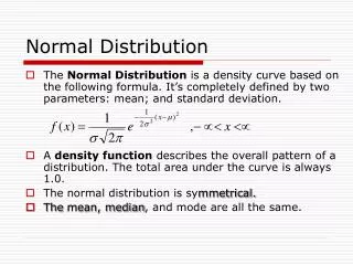
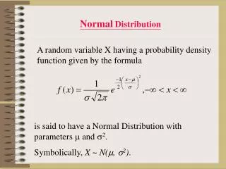
2. Normal distributions are a family of distributions that have the same general shape. • They are symmetric with scores more concentrated in the middle than in the tails • Normal distributions are sometimes described as bell shaped. • The area under each curve is the same. • The height of a normal distribution can be specified mathematically in terms of two parameters: the mean ( ) and the standard deviation ( ). • The height (ordinate) of a normal curve is defined as:

3. Equation

4. Features • It is bell-shaped • It is symmetrical about the mean • It extends from -∞ to +∞ • The total area under the curve is 1 • The maximum value of f(x) is

5. Approximately 95% of the distribution lies within two standard deviations from the mean.

6. Approximately 99.9% of the distribution lies within three standard deviations from the mean.

7. The shape depends on the value of

8. Definition The standard normal distribution is a normal distribution with a mean of 0 and a standard deviation of 1

9. Normal distributions can be transformed to standard normal distributions by the formula: where X is a score from the original normal distribution,   is the mean of the original normal distribution, and is the standard deviation of original normal distribution.

10. The standard normal distribution is sometimes called the z distribution. A z score always reflects the number of standard deviations above or below the mean a particular score is.

11. For instance, if a person scored a 70 on a test with a mean of 50 and a standard deviation of 10, then they scored 2 standard deviations above the mean. Converting the test scores to z scores, an X of 70 would be:So, a z score of 2 means the original score was 2 standard deviations above the mean. Note that the z distribution will only be a normal distribution if the original distribution (X) is normal.

12. Applying the formula will always produce a transformed distribution with a mean of zero and a standard deviation of one. However, the shape of the distribution will not be affected by the transformation.

13. Using the chart • Need to know how many standard deviations you are from the mean. • Use

14. Readings can be made to the left ‘P’ (Chart 0.5 +)

15. Readings can be made to the left ‘P’ (Chart 0.5 +)

16. To the centre ‘Q’

17. To the centre ‘Q’

18. Or to the right ‘R’ (Chart 0.5 - x)

19. Or to the right ‘R’ (Chart 0.5 - x)

20. Lengths of metal strips produced by a machine are normally distributed with a mean length of 150 cm and a standard deviation of 10 cm. • Find the probability that the length of a randomly selected strip is shorter than 165 cm.

21. Lengths of metal strips produced by a machine are normally distributed with a mean length of 150 cm and a standard deviation of 10 cm. • Find the probability that the length of a randomly selected strip is within 5 cm of the mean 150

22. The time taken by the milkman to deliver to the High Street is normally distributed with a mean of 12 mins and standard deviation of 2 mins. He delivers milk every day. • Estimate the number of days during the year when he takes longer than 17 mins. 12 Two days

23. The time taken by the milkman to deliver to the High Street is normally distributed with a mean of 12 mins and standard deviation of 2 mins. He delivers milk every day. • Estimate the number of days during the year when he takes less than ten mins. 12 58 days

24. The time taken by the milkman to deliver to the High Street is normally distributed with a mean of 12 mins and standard deviation of 2 mins. He delivers milk every day. • Estimate the number of days during the year when he takes between nine and 13 mins. 228 days 12

25. Inverse Normal

26. Given that 80% of these female students have a height less than h cm, find the value of h. Given that 60% of these female students have a height greater than s cm, find the value of s. The heights of female students at a particular school are normally distributed with a mean of 169 cm and a standard deviation of 9 cm

27. z = 0.842 169 h

28. z = 0.253 s 169

29. Batteries for a transistor radio have a mean life under normal usage of 160 hours, with a standard deviation of 30 hours. Assuming a normal distribution: • Calculate the percentage of batteries which have a life between 150 hours and 180 hours. 37.8%

30. Batteries for a transistor radio have a mean life under normal usage of 160 hours, with a standard deviation of 30 hours. Assuming a normal distribution: • Calculate the range, symmetrical about the mean, within which 75% of the battery lives lie. 125.5, 194.5

31. The masses of boxes of oranges are normally distributed such that 30% of them are greater than 4.00 kg and 20% are greater than 4.53 kg. Estimate the mean and standard deviation of the masses. 3.13, 1.67

32. The speeds of cars passing a certain point on a motorway can be taken to be normally distributed. Observations show that of cars passing the point, 95% are travelling at less than85 kph and 10% are travelling at less than 55 kph. • Find the average speed of the cars passing the point. 68 kph

33. The speeds of cars passing a certain point on a motorway can be taken to be normally distributed. Observations show that of cars passing the point, 95% are travelling at less than85 kph and 10% are travelling at less than 55 kph. • Find the proportion of cars that travel at more than 70 kph. 0.4282

34. Sometimes the normal distribution (a continuous distribution) is used to approximate situations that are really discrete. This occurs when data is measured to the nearest whole number. • The distribution takes on the shape of a normal distribution. In fact, the normal curve was instigated by De Moivre as an approximation to the Binomial.

35. The discrete data is represented by its limits • E.g. 7 becomes the interval

36. Normal Approximation to the Binomial Distribution

37. Notice that as N increases, the binomial distribution approximate to a normal distribution.

38. Binomial distributions N = 5, p = 0.5 N = 5, p = 0.2 N = 10, p = 0.2 N = 10, p = 0.5

39. Binomial distributions N = 20, p = 0.2 N = 20, p = 0.5 N = 30, p = 0.2 N = 30, p = 0.5

40. The binomial distribution can be approximated by a normal distribution under the conditions

41. Careful of the language • As a Binomial is a discrete distribution, a continuity correction is necessary. • P(at most 3) • P(fewer than 3) • P(exactly 3) • P(more than 3) • P(at least 3)

42. Example • It is given that 40% of the population support the Gambage Party. 150 members of the population are selected at random. Use a suitable approximation to find the probability that more than 55 out of these 150 support the Gambage Party.

43. It is given that 40% of the population support the Gambage Party. 150 members of the population are selected at random. Use a suitable approximation to find the probability that more than 55 out of these 150 support the Gambage Party. • Binomial distribution • N = 150, p = 0.4 • Np = 60 • Np(1-p) = 90 • Use a normal distribution

44. Normal approximation to the Poisson distribution

45. Notice as values ofincrease, the distribution becomes normally distributed.

46. As lambda increase, the normal approximation gets better.

47. We use the criteria

48. Poisson is a discrete distribution and hence we need to use a continuity correction

49. The number of bacteria on a plate follows a Poisson distribution with a parameter 60. Find the probability that there are between 55 and 75 bacteria on a plate.

50. The number of bacteria on a plate follows a Poisson distribution with a parameter 60. Find the probability that there are between 55 and 75 bacteria on a plate.