ANCOVA
ANCOVA. Group 4. AMS 572. Table of Contents. 1. Introduction and History 1.1 Part 1: Ahram Woo 1.2 Part 2: Jingwen Zhu 2 . Theoretical Background 2.1 Part 1: Xin Yu 2.2 Part 2: Unjung Lee 3. Application of ANCOVA and Summary 3.1 Part 1: Xiaojuan Shang

ANCOVA
E N D
Presentation Transcript
ANCOVA Group 4 AMS 572
Table of Contents 1. Introduction and History 1.1 Part 1: Ahram Woo 1.2 Part 2: Jingwen Zhu 2. Theoretical Background 2.1 Part 1: Xin Yu 2.2 Part 2: Unjung Lee 3. Application of ANCOVA and Summary 3.1 Part 1: Xiaojuan Shang 3.2 Part 2: YoungaChoi 3.3 Part 3: Qiao Zhang
1. Introduction and History Group 4 by Ahram Woo
1. Introduction and History Individual by Ahram Woo Xin Yu Ahram Woo Unjung Lee Jingwen Zhu Qiao Zhang Xiaojuan Shang YoungaChoi
1. Introduction and History 1.1 Introduction to ANCOVA by Ahram Woo • Analysis of covariance : An extension of ANOVA in which main effects and interactions are assessed on Dependent Variable(DV) scores after the DV has been adjusted for by the DV’s relationship with one or more Covariates (CVs) • ANCOVA = ANOVA + Linear Regression
1. Introduction and History 1.1 Introduction to ANCOVA by Ahram Woo • R.A. Fisher who is credited with the introduction of ANCOVA "Studies in crop variation. IV. The experimental determination of the value of top dressings with cereals" published in Journal of Agricultural Science, vol. 17, 548-562. The paper was published in 1927.
1. Introduction and History 1.1 Introduction to ANCOVA by Ahram Woo • ANOVA is described by R. A. Fisher to assist in the analysis of data from agricultural experiments. • ANOVA compare the means of any number of experimental conditions without any increase in Type 1 error. • ANOVA is a way of determining whether the average scores of groups differed significantly.
1. Introduction and History 1.2 Introduction to Linear Regression by Jingwen Zhu Model the relationship between explanatory and dependent variables by fitting a linear equation to observed data. (i.e. Y = a + bX) • There is a relationship or not ? • One variable causes the other? • Scatter Plot & Correlation Coefficient
1. Introduction and History 1.2 Introduction to Linear Regression by Jingwen Zhu The term “ regression” was first studied in depth by 19th-century scientist, Sir. Francis Galton. • Geographer • Psychologist • Statistician • Meteorologist • Eugenicist
1. Introduction and History 1.2 Introduction to Linear Regression by Jingwen Zhu Galton studied data on relative heights of fathers and their sons Conclusions: • A taller-than-average father tends to produce a taller-than-average son • The son is likely to be less tall than the father in terms of his relative position within his own population
1. Introduction and History 1.2 Introduction to Linear Regression by Jingwen Zhu • ANCOVA is a merger of ANOVA and regression. • ANCOVA allows to compare one variable in 2 or more groups taking into account (or to correct for) variability of other variables, called covariates. • The inclusion of covariates can increase statistical power because it accounts for some of the variability
1. Introduction and History 1.2 Introduction to Linear Regression by Jingwen Zhu Example: whether MCAT scores are significantly different among medical students who had different types of undergraduate majors, when adjusted for year of matriculation? • Dependent variable (continuous) • MCAT total (most recent) • Fixed factor (categorical variables) • Undergraduate major • 1 = Biology/Chemistry • 2 = Other science/health • 3 = Other • Covariate • Year of matriculation
1. Introduction and History 1.2 Introduction to One-way Analysis of Variance by Jingwen Zhu • One factor of k levels or groups. E.g., 3 treatment groups in a drug study. • The main objective is to examine the equality of means of different groups. • Total variation of observations (SST) can be split in two components: variation between groups (SSA) and variation within groups (SSE).
1. Introduction and History 1.2 Introduction to One-way Analysis of Variance by Jingwen Zhu Consider a layout of a study with 16 subjects that intended to compare 4 treatment groups (G1-G4). Each group contains four subjects. S1 S2 S3 S4 G1 Y11 Y12 Y13 Y14 G2 Y21 Y22 Y23 Y24 G3 Y31 Y32 Y33 Y34 G4 Y41 Y42 Y43 Y44
1. Introduction and History 1.2 Introduction to One-way Analysis of Variance by Jingwen Zhu • Model: • Assumptions: • Observations yij are independent. • are normally distributed with mean zero and constant standard deviation.
1. Introduction and History 1.2 Introduction to One-way Analysis of Variance by Jingwen Zhu • Hypothesis Ho: Means of all groups are equal. Ha: At least one of them is not equal to other. • ANOVA Table
1. Introduction and History 1.2 Introduction to One-way Analysis of Variance by Jingwen Zhu SSA (Variation between groups)is due to the difference in different groups. E.g. different treatment groups or different doses of the same treatment.
1. Introduction and History 1.2 Introduction to One-way Analysis of Variance by Jingwen Zhu
1. Introduction and History 1.2 Introduction to One-way Analysis of Variance by Jingwen Zhu SSE (Variation within groups) is the inherent variation among the observations within each group.
1. Introduction and History 1.2 Introduction to One-way Analysis of Variance by Jingwen Zhu
1. Introduction and History 1.2 Introduction to One-way Analysis of Variance by Jingwen Zhu • SST (SUM SQUARE OF TOTAL) is the combination of SSE and SSA
Data, the Grand Error N(0, ^2) σ jth mean of Y observatio Effects of the jth group(we mainly n of the ith focus on when ai=0,i=1, … ,a ) group 2. Theoretical Background 2.1 Model of ANOVA by Xin Yu
Data, the Error Predictor (ij)th observation Slope and Intersect (we mainly focus on the estimate) 2. Theoretical Background 2.1 Model of Linear Regression by Xin Yu
Effects of the ith Known covariance group (We still focus on if ai=0, i=1, … ,a) 2. Theoretical Background 2.1 ANCOVA: ANOVA Merged With Linear Regression by Xin Yu
2. Theoretical Background 2.1 How to Perform ANCOVA by Xin Yu ANOVA Model!
2. Theoretical Background 2.1 How do we get by Xin Yu Within each group, consider ai as a constant, and notice that we actually only desire the estimate of slope β instead of intersect.
2. Theoretical Background 2.1 How do we get (continue) by Xin Yu (*)Within each group, do Least Square: (*)Assume that β1=…=βi=…=βa (*)Which means that αi and β are independent; Or, Covariate has nothing to do with group effect
2. Theoretical Background 2.1 How do we get (continue) by Xin Yu We use POOLED ESTIMATE of β
2. Theoretical Background 2.1 Model of ANOVA by Xin Yu
2. Theoretical Background 2.2.A The Simple Linear Regression Model by Unjung Lee Y = β0 + β1 X+ ε Y : dependent (response) variable X : independent (predictor) variable β0 : the intercept β1 : the slope ε : error term ~ N(0,σ2) E(Y) = β0 + β1X
2. Theoretical Background 2.2.A The Simple Linear Regression Model by Unjung Lee Y E(Y) =β0 + β1x { y } } Error: β1 = Slope 1 β0 = Intercept X
2. Theoretical Background 2.2.A The Simple Linear Regression Model by Unjung Lee Y E(Y) =β0 + β1x y Identical normal distributions of errors, all centered on the regression line. N(my|x,sy|x2)
2. Theoretical Background 2.2.A Assumptions of simple linear regression model by Unjung Lee • The relationship between X and Y is the straight-line relationship. • X and Y has a common variance σ2 . • Error is normally distributed. • Error is independent.
2. Theoretical Background 2.2.A The least squares(LS) method by Unjung Lee
2. Theoretical Background 2.2.A The least squares(LS) method by Unjung Lee The fitted values and residuals We can get these ones with the normal equations
2. Theoretical Background 2.2.A Fitting a Regression Line by Unjung Lee Y Y Data Three errors from the least squares regression line X X Y e Errors from the least squares regression line are minimized Three errors from a fitted line X X
2. Theoretical Background 2.2.A Errors in Regression by Unjung Lee Y . yi { X xi
2. Theoretical Background 2.2.A Multiple linear regression by Unjung Lee A statistical model that utilizes two or more quantitative and qualitative explanatory variables (x1,..., xp) to predict a quantitative dependent variable Y. Caution: have at least two or more quantitative explanatory variables (rule of thumb)
2. Theoretical Background 2.2.A Dummy-Variable Regression Model by Unjung Lee • Involves categorical X variable with two levels • e.g., female-male, employed-not employed, etc. • Variable levels coded 0 & 1 • Assumes only intercept is different • Slopes are constant across categories
2. Theoretical Background 2.2.A Dummy-Variable Model Relationships by Unjung Lee Y Same slopes b1 Females b0 + b2 b0 Males 0 X1 0
2. Theoretical Background 2.2.A Dummy Variables by Unjung Lee • Permits use of qualitative data (e.g.: seasonal, class standing, location, gender). • 0, 1 coding (nominative data) • As part of Diagnostic Checking; incorporate outliers (i.e.: large residuals) and influence measures.
2. Theoretical Background 2.2.A Interaction Regression Model by Unjung Lee • Hypothesizes interaction between pairs of X variables • Response to one X variable varies at different levels of another X variable • Contains two-way cross product terms Y = 0 + 1x1 + 2x2 + 3x1x2 + • Can be combined with other models e.g. dummy variable models
2. Theoretical Background 2.2.A Effect of Interaction by Unjung Lee • Given: • Without interaction term, effect of X1 on Y is measured by 1 • With interaction term, effect of X1 onY is measured by 1 + 3X2 • Effect increases as X2i increases β β β
2. Theoretical Background 2.2.A Interaction Example by Unjung Lee Y = 1 + 2X1 + 3X2 + 4X1X2 Y Y = 1 + 2X1 + 3(1) + 4X1(1) = 4 + 6X1 12 8 Y = 1 + 2X1 + 3(0) + 4X1(0) = 1 + 2X1 4 0 X1 0 0.5 1 1.5 Effect (slope) of X1 on Y does depend on X2 value
2. Theoretical Background 2.2.A The two-way ANOVA by Unjung Lee
2. Theoretical Background 2.2.A The two-way ANOVA table by Unjung Lee
2. Theoretical Background 2.2.A Test homogeneity of variance by Unjung Lee
2. Theoretical Background 2.2.B Test Whether Ho: by Xin Yu
2. Theoretical Background 2.2.B Test Whether Ho: by Xin Yu (1) Define Sum of Square of Errors within Groups Is calculated based on AND, is generated by the random error ε.
2. Theoretical Background 2.2.B Test Whether Ho: by Xin Yu (2) SSE is generated by (*) Random Error ε (*)Difference between distinct we can calculate SSE based on a common (3) Let SSA=SSE- SSA Sum of Square between Groups SSA is constituted by the difference between different