ANCOVA
ANCOVA. ANCOVAphiles & GLMers & Regressionists Workings of ANOVA & ANCOVA ANCOVA, Semi-Partial correlations, statistical control Using model plotting to think about ANCOVA & Statistical control Homogeneity & Heterogeneity of Regression slope .

ANCOVA
E N D
Presentation Transcript
ANCOVA • ANCOVAphiles & GLMers & Regressionists • Workings of ANOVA & ANCOVA • ANCOVA, Semi-Partial correlations, statistical control • Using model plotting to think about ANCOVA & Statistical control • Homogeneity & Heterogeneity of Regression slope
It’s all OLSGLM – “But be careful where you say that, friend!” Most of the statistical models (excluding some of the “nonparametric” ones) you know have been applied, advanced, improved, integrated, separated, named and renamed by a plethora of research areas, resulting in, well… a real mess… • There are 3 (main) parts to this: • General Linear Model • Expressing all models as linear combinations of linearly weighted variables (including coded categorical, nonlinear & interactions terms, etc & their combinations) • Distributional assumptions & robustnesses • Multivariate normal distributions • Various “homogeneities” (variance, covariance, slope) • Defining “best fitting model” • OLS or “ordinary least squares” min ∑(y-y’)2
There have been multiple attempts to reintegrate the “various named things” under a single central model… The nice folks over in “math stats” have long recognized that these are varieties and variations of a single math model. But, different research areas have “acquired” the models in different orders, for different reasons, from different sources, allowing different “acceptable variations” and, perhaps most importantly…. … calling them different things ... developing software to perform them that accepts different inputs, produces different outputs and labels things differently! Combine this with “market considerations” & a tendency not to change software but rather to add new things with new names whenever a competitor adds new things & you get the current mess….
In psychology (& friends) there have been 2 “paths to GLM” • Path #1 ANOVA &Enhanced ANOVA • Experimentalists used ANOVA • Categorical IVs (mostly – but rem “trend analyses” for “parametric designs with quant IVs) • Always included main effect & interactions among IVs • With the increase in non-Experimental designs, there was an increased use of ANCOVAto provide statistical control • Categorical IVs & (usually) quantitative “Covariates” (confounds, controls, etc) • Always included main effects & interactions among IVs • Assumed (hoped for) homogeneity of regression slope – just the main effects of the covariates • Grudgingly tolerated interactions with and among covariates (“failure of regression homogeneity”)
Path #2 Regression&Enhanced Regression • NonexperimentalistsusedRegression • Quantitative predictors (mostly – but figured out that binary predictors have the same interpretation) • Linear main effects models (steadfastly!!!!) • Unique contribution of each variable “controlling for others” • Need Enhancements to allow inclusion other variable types & comparisons… • Multiple-category variables (coding) • Nonlinear terms ( X2 ) • Interactions • Comparison of nested models (linear vs “embelishments”) • Either “path” gets you to GLM • All the variable types • Interactions • Unique contributions controlling for other variables in model
So, today we’re gonna talk about ANCOVA as… … ANOVA with “enhancements” Instead of asking… “What is the mean DV difference between the groups assuming the only difference between the groups is the IV?” We’re gonna ask… “What is the mean DV difference between the groups, holding the value of one or more covariates constant at specified values?”
You know how ANOVA works • the total variation among a set of scores on a quantitative variable is separated into between groups and within groups variation • between groups variation reflects the extent of the bivariate relationship between the grouping variable and the quant variable -- systematic variance • within groups variation reflects the extent that variability in the quant scores is attributable to something other than the bivariate relationship -- unsystematic variance • F-ratio compares these two sources of variation, after taking into account the number of sources of variability • dfbg-- # groups - 1 • dfwg -- # groups * (number in each group -1) • the larger the F, the greater the systematic bivariate relationship
ANCOVA allows the inclusion of a 3rd source of variation into the F-formula (called the covariate) and changes the F-formula Loosely speaking… BG variation attributed to IV ANOVA Model F = ----------------------------------------------------- WG variation attributed to individual differences BG variation BG variation attributed to IV + attributed to COV ANCOVA F = ----------------------------------------------------------------- WG variation attributed + WG variation attributed to individual differences to COV
Imagine an educational study that compares two types of spelling instruction. Students from 3rd, 4th and 5th graders are involved, leading to the following data. Control Grp Exper. Grp S1 3rd 75 S2 4th 81 S3 3rd 74 S4 4th 84 S5 4th 78 S6 5th 88 S7 4th 79 S8 5th 89 • Individual differences (compare those with same grade & grp) • compare Ss 1-3, 5-7, 2-4, 6-8 • Treatment (compare those with same grade & different grp) • compare 5,7 to 2,4 Grade (compare those with same group & different grade) compare 1,3 to 5,7 or 2,4 to 6,8 • Notice that Grade is: • acting as a confound – will bias estimate of the treatment effect • acting to increase within-group variability – will increase error
ANOVA • ignores the covariate • attributes BG variation exclusively to the treatment • but BG variation actually combines Tx & covariate • attributes WG variation exclusively to individual differences • but WG variation actually combines ind difs & covariate • F-test of Tx effect “ain’t what it is supposed to be” • ANCOVA • considers the covariate (a multivariate analysis) • separates BG variation into Tx and Cov • separates WG variation into individual differences and Cov • F-test of the TX effect while controlling for the Cov, using ind difs as the error term • F-test of the Cov effect while controlling for the Tx, using ind difs as the error term
ANCOVA is the same thing as a semi-partial correlation between the IV and the DV, correcting the IV for the Covariate • Applying regression and residualization as we did before … • predict each person’s IV score from their Covariate score • determine each person’s residual (IV - IV’) • use the residual in place of the IV in the ANOVA (drop 1 error df) • The resulting ANOVA tells the relationship between the DV and IV that is unrelated to the Covariate • OR... • ANCOVA is the same thing as multiple regression using both the dummy coded IV and the quantitative covariate as predictors of the DV • the “b” for each shows the relationship between that predictor and the DV, controlling the IV for the other predictor • OR… • ANCOVA is a particular version of GLM
Several things to remember when applying ANCOVA: • H0: for ANOVA & ANCOVA are importantly different • ANOVA: No mean difference between the populations represented by the treatment groups. • ANCOVA: No mean difference between the populations represented by the treatment groups, assuming all the members of both populations have a covariate score equal to the overall covariate mean of the current sampled groups. • Don’t treat statistical control as if it were experimental control • You don’t have all the confounds/covariates in the model, so you have all the usual problems of “underspecified models” • The underlying philosophy (or hope) of ANCOVA, like other multivariate models is, “Behavior is complicated, so more complicated models, will on average, be more accurate.” • Don’t confuse this with, “Any given ANCOVA model is more accurate than the associated ANOVA model.”
As you can see, there are different “applications” of ANCOVA • “correcting” the assessment of the IV-DV relationship for within group variability attributable to the covariate • will usually increase F -- by decreasing the “error variation? • “correcting” the assessment of the IV-DV relationship for between group variability attributable to the covariate • will increase or decrease F by increasing or decreasing the “Tx effect” -- depending upon whether covariate and Tx effects are in “same” or “opposite” directions • “correcting” for both influences of the covariate upon F • F will change as a joint influence of decreasing “error variation” and increasing/decreasing “systematic variation” • You should recognize the second as what was meant by “statistical control” when we discussed that topic in the last section of the course
How a corresponding ANOVA & ANCOVA differ… • SSerror for ANCOVA will always be smaller than SSerror for ANOVA • part of ANOVA error is partitioned into covariate of ANCOVA • SSIV for ANCOVA may be =, < or > than SSIV for ANOVA • depends on the “direction of effect” of IV & Covariate • Simplest situation first! • Case #1: If Tx = Cx for the covariate (i.e., there is no confounding) • ANOVA SSIV= ANCOVA SSIV there’s nothing to control for • smaller SSerror– So F will be larger & more sensitive • F-test for Tx may still be confounded by other variables
If Tx ≠Cx for the covariate (i.e., there is confounding) • ANOVA SSIV ≠ ANCOVA SSIV • we can anticipate the ANOVA-ANCOVA difference if we pay attention to the relative “direction” of the IV effect and the “direction” of confounding • Case #2: if the Tx & Confounding are “in the opposite direction” • eg, the 3rd graders get the Tx (that improves performance) and 5th graders the Cx • ANOVA will underestimate the TX effect (combining Tx & the covariate into the SSIV • ANCOVA will correct for that underestimation (partitioning Tx & covariate into separate SS) • ANOVA SSIV< ANCOVA SSIV • smaller SSerror • F-tests for Tx and for Grade will be “better” – but still only “control” for this one covariate (there are likely others) ANCOVA F > ANOVA F
Case #3: if the Tx & Confounding are “in the same direction” • eg, the 5th graders get the Tx (that improves performance) and 3rd graders the Cx • ANOVA will overestimate the TX effect (combining Tx & the covariate into the SSIV • ANCOVA will correct for that overestimation (partitioning Tx & covariate into separate SS) • ANOVA SSIV> ANCOVA SSIV • smaller SSerror • Can’t anticipate whether F from ANCOVA or from ANOVA will be larger – ANCOVA has the smaller numerator & also the smaller denominator • F-tests for Tx and for Grade will be “better” – but still only “control” for this one covariate (there are likely others)
Since we’ve recently learned about plotting … How do the plots of ANOVA & ANCOVA differ and what do we learn from each? Here’s a plot of a 2-group ANOVA model Z = Tx1 vs. Cx Cx = 0Tx = 1 y’ = bZ + a Tx b is our estimate of the treatment effect 0 10 20 30 40 50 60 b Cx
Here’s a plot of the corresponding 2-group ANCOVA model … … … with no confounding by “X” for mean Xcen Cx = Tx So, when we use ANCOVA to hold Xcen constant at 0 we’re not changing anything, because there is no X confounding to control, “correct for” or “hold constant. Z = Tx1 vs. Cx Cx = 0Tx = 1 Tx Xcen = X – Xmean b2 0 10 20 30 40 50 60 b is a good estimate of the treatment effect Cx -20 -10 0 10 20 Xcen
Here’s a plot of the corresponding 2-group ANCOVA model … … with confounding by “X” for mean XcenCx < Tx When we compare the mean Y of Cx & Tx using ANOVA, we ignore the group difference/confounding of X – and get a biased estimate of the treatment effect When we use ANCOVA to compare the groups -- holding Xcen constant at 0 -- we’re controlling for or correcting the confounding and get a better estimate of the treatment effect. Here the corrected treatment effect is smaller than the uncorrected treatment effect. Z = Tx1 vs. Cx Cx = 0Tx = 1 Tx Xcen = X – Xmean b2 0 10 20 30 40 50 60 b is our estimate of the treatment effect Cx -20 -10 0 10 20 Xcen
Here’s a plot of the corresponding 2-group ANCOVA model … … with confounding by “X” for mean XcenCx > Tx When we compare the mean Y of Cx & Tx using ANOVA, we ignore the group difference/confounding of X – and get a biased estimate of the treatment effect When we use ANCOVA to compare the groups -- holding Xcen constant at 0 -- we’re controlling for or correcting the confounding and get a better estimate of the treatment effect. Here the corrected treatment effect is larger than the uncorrected treatment effect. Z = Tx1 vs. Cx Cx = 0Tx = 1 Tx Xcen = X – Xmean b2 0 10 20 30 40 50 60 b is our estimate of the treatment effect Cx -20 -10 0 10 20 Xcen
The “regression slope homogeneity assumption” in ANCOVA • You might have noticed that the 2 lines representing the Y-X relationship for each group in the ANCOVA plots were always parallel – had the same regression slope. • these are main effects ANCOVA models that are based on… • the homogeneity of regression slope assumption • the reason it is called an “assumption” is that when constructing the main effects model we don’t check whether or not there is an interaction, be just build the model without an “interaction term” – so the lines are parallel (same slope) • There are two consequences of this assumption: • Y & X have the same relationship/slope for both groups • the group difference on Y is the same for every value of X • REMEMBER neither of these are “discoveries” they are both assumptions
If forsake the homogeneity of regression slope assumption, we… • Include an interaction term in the model • Allow the DV-Covariate regression lines for each group to be nonparellel • The direction and size of the group difference depends upon the value of the covariate we “hold constant at” Raw or “uncorrected” group difference Tx Corrected group difference at X= 0 Corrected group difference at X= -10 0 10 20 30 40 50 60 Corrected group difference at X= 15 Cx -20 -10 0 10 20 Xcen
But what if, you may ask, there are more than one “confound” you want to control for? • Just “expand” the model … • SSIV + SScov1 + … + SScovk • SStotal = ------------------------------------------ • SSError • You get an F-test for each variable in model … • You get a b, β & t-test for each variable in model … • Each of which is a test of the unique contribution of that variable to the model after controlling for each of the other variables • Remember: ANCOVA is just a multiple regression with one categorical predictor called “the IV”