Difference Between the Means of Two Populations
140 likes | 424 Vues
Difference Between the Means of Two Populations . We have be studying inference methods for a single variable. When the variable was quantitative we had inference for the population mean. When the variable was qualitative we had inference for the population proportion.

Difference Between the Means of Two Populations
E N D
Presentation Transcript
We have be studying inference methods for a single variable. When the variable was quantitative we had inference for the population mean. When the variable was qualitative we had inference for the population proportion. Now we want to study inference methods for two variables. Both variables could be quantitative, both qualitative or one of each. Depending on the which we have, we will look to certain techniques. At this stage of the game we will begin to look at these different methods. I want to start with 1 quantitative variable and one qualitative variable. In fact the qualitative variable is special here: the variable identifies membership in one of only two groups. Then on the quantitative variable we segment each observation into the appropriate group and think about the mean of the quantitative variable of each group.
Our context here is that we really want to know about the population of the two groups, but we will only take a sample from each group. We will look at both confidence intervals and hypothesis tests in this context. Some notation: μi = the population mean of group i for i = 1, 2. σi = the population standard deviation for group i for i = 1, 2. xi = the sample mean of group i for i = 1, 2. si = the sample standard deviation for group i for i = 1, 2. Now for ease of typing I will call the population means mu1 or mu2, population standard deviations sigma1 or sigma2, sample means xbar1 or xbar2, and sample standard deviations s1 or s2. n1 is the sample size from population 1 and n2 has similar meaning.
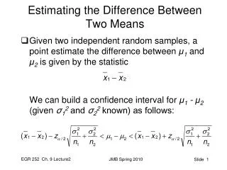
Our context for inference is really the difference in means: mu1 minus mu2. So we are checking to see what difference there is in the means from the two groups. Our point estimator will be xbar1 minus xbar2. In a repeated sampling context the point estimator would vary from sample to sample. As an example say I want to check the average age of students in the economics program and the finance program. One sample from each group would yield one estimate and the estimate would likely be different when I get a different sample (from each major). Also note the sample obtained from group 1 is independent of the sample obtained from group 2. The sampling distribution of xbar1 minus xbar2 will be studied next.
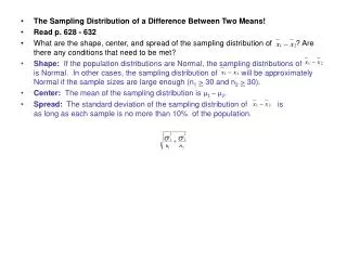
The sampling distribution of xbar1 minus xbar2 Case 1 – we can use the normal distribution for the sampling distribution when sigma1 and sigma2 are known. This means we will use Z in our confidence intervals and hypothesis tests The center of the sampling distribution is mu1 minus mu2 and the standard error is the (note or digress x^2 means x squared ) square root[((sigma1^2)/n1)+((sigma2^2)/n2)]. Case 2 – we can use the t distribution for the sampling distribution when sigma1 and sigma2 are unknown. This means we will use t in our confidence intervals and hypothesis tests. The center of the sampling distribution is mu1 minus mu2 and the standard error is seen as the denominator of equation 10.2 on page 313. This is not pretty, but we must use it. Note that when using a t distribution one needs to have a degrees of freedom value. In our current context the value is n1 + n2 – 2.
Inference for case 1 Confidence interval We are C% confident the unknown population difference mu1 minus mu2 is in the interval (xbar1 minus xbar2) ± MOE, Where MOE = margin of error and this equals the appropriate Z times the standard error of the sampling distribution. Remember if C = 95 the Z = 1.96, and if C = 90 the Z = 1.645, and if C = 99 the Z = 2.58.
Hypothesis Test Recall from our past work that in an hypothesis test context we have a null and an alternative hypothesis. Plus the form of the alternative hypothesis will determine if we have a one or a two tailed test. Two tailed test When we study the difference in the means from two populations if we feel there is a difference of Do, but not concerned about the difference being positive or negative, then the null and alternative hypotheses are Ho: mu1 minus mu2 = Do, Ha: mu1 minus mu2 ≠ Do, and we have a two tailed test. Based on an alpha value (the probability of a type I error), we pick critical values of Z and if the calculated Z is more extreme than either critical value we reject the null and go with the alternative.
Alpha/2 alpha/2 lower Critical Z Upper Critical Z The calculated value of Z from the sample information = [(xbar1 minus xbar2) minus Do] divided by the standard error listed on slide 5 with case 1. Another way to think of the hypothesis test is with the use of the p-value for the calculated Z. If the p-value < alpha, reject the null. Otherwise you have to stick with the null. In practice with a two tailed test you will find the p-value as the area on one side of the distribution but you must double it to be on both sides.
One tailed test When the researcher has the feeling that the difference in mu1 and mu2 should be positive, then the alternative will reflect this feeling and we will have Ho: mu1 minus mu2 ≤ Do Ha: mu1 minus mu2 > Do. The signs are reversed when the researcher feels the difference should be negative. The test procedure proceeds in the same fashion as with the two-tailed test except the focus is just on one side of the distribution as directed by the alternative hypothesis. Note that Do is often zero. In that case we just want to see if the group means are different.
Common critical Z’s Two tailed test One tailed test (negative if on left) Alpha = .05 1.96 1.645 Alpha = .01 2.58 2.326 Alpha = .10 1.645 1.282
Problems 1, 2, 3 page 319 • Zstat = (72 - 66 – 0)/SQRT[((20^2)/40) + ((10^2)/50)] = 6/sqrt[(400/40) + (100/50)] = 6/sqrt(12) = 1.73 • 2) With alpha = .01 with a two tailed test we have .01/2 on each side. The critical Z’s would have .005 in each tail. So we have critical Z’s of -2.58 and 2.58. Since 1.73 is in the middle we do not reject the null. So, we have to say the population means are equal. • 3) The tail area for Z = 1.73 is (1- .9582) = .0418 and we double because of two tail test for a p-value of .0836. Since this is greater than .01 we can not reject the null.
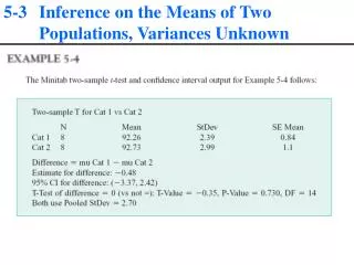
Inference for case 2 Inference for case 2 is similar to case 1, except in how the standard error is calculated and that is shown on slide 5 and in using t. Let’s do problem 4 page 319 a) Looking at page 313 let’s first calculate the S squared sub p amount [(7)16 + (14)25]/21 = [112 + 350]/21 = 22 The tstat = [42 - 34 – 0]/sqrt[22((1/8) + (1/15)) = 8/sqrt((22)(23/120)) = 8/2.05 = 3.90 (book answer is different due to rounding) b) Df = n1 + n2 – 2 = 8 + 15 – 2 = 21 c) Critical t from the table is 2.5177. d) Since our tstat 3.90 > 2.5177 we reject the null and conclude mu1 > mu2.
Problem 8 page 320 a) Let’s say mu1 = mean strength of the new machine and mu2 = mean strength old machine. Ho: mu1 ≤ mu2 H1: mu1 > mu2. With a one tail test (upper tail) the critical Z (use Z because population standard devs are known) with alpha = .01 is 2.33. The Zstat from the sample information is (72 – 65 – 0)/sqrt[((81/100) + ((100/100))] = 7/sqrt(181/100) = 5.20. This is more extreme than the critical value so we reject the null. There is evidence to get the new machine. b) The Zstat = 5.20 has p-value (upper tail) approximately = .0000003 which is < .01. Reject null.
Problem 12 page 321 a) Let’s say mu1= mean score for men and mu2= mean score for women. Ho: mu1 = mu2 H1: mu1 ≠ mu2. With a two tail test the critical t’s (use t because population standard devs are UNknown) with alpha = .05 and df = 170 are -1.9799 and 1.9799 (df = 120 is as close as we can get!!!) The S squared sub p in the formula is [99(13.35)^2 + 71(9.42)^2]/[99+71] = 140.85. The tstat from the sample information is (40.26 – 36.85 – 0)/sqrt[140.85((1/100) + ((1/72))] = 3.41/1.83 = 1.86. This is between the critical values so we can not reject the null. The evidence suggests the population means are the same for males and females. b) The tstat = 1.86 has upper tail between .025 and .05 and doubling for two tail test p-value is between .05 and .10 which is > .05. Do not reject null.