Optimizing Prefix Adders and Division Algorithms for Efficient FPGA Implementation
This document explores the evaluation and advancements in prefix adders, specifically analyzing well-known architectures such as Sklansky, Kogge-Stone, and Brent-Kung. It discusses realistic design considerations including timing, power consumption, and area requirements. The role of integer linear programming and logic effort timing models is examined for effective optimization. Additionally, it presents division techniques using the PST algorithm suitable for high-performance FPGA designs, detailing methods like series expansion and pre-scaling to enhance operational efficiency while addressing memory and arithmetic efforts.


Optimizing Prefix Adders and Division Algorithms for Efficient FPGA Implementation
E N D
Presentation Transcript
Datapath Designs CK Cheng CSE Department UC, San Diego
Prefix Adder –Well-known and Well-developed? • Classic prefix networks: Sklansky, Kogge-Stone, Brent-Kung, Ladner-Fischer, Han-Carlson, Knowles etc.
Prefix Adder –New Respects, New Method • Realistic design considerations: Timing, Power and Area. • Integer Linear Programming for prefix adder: • Logic effort timing model (gate cap. + wire cap.) • Activity-statistic power model • Non-uniform signal arrival/required times Logic Levels Timing Power Area Max Fanouts Max Wire Tracks
Prefix Adder –Optimum Prefix adders • Uniform signal arrival/required times Sklansky Adder Kogge-Stone Adder Fastest depth-3 optimal prefix adder Fastest depth-4 optimal prefix adder
Prefix Adder –Optimum Prefix adders • Uniform signal arrival/required times
Prefix Adder –Optimum Prefix adders • Non-uniform signal arrival/required times Increasing Signal Arrival Times Decreasing Signal Arrival Times Convex Signal Arrival Times
0.1 1 0 1 1 0 1 0 1 0 0 1 R0=A 1 0 1 0 1 0 0 0 R1 Q1 = 0.1Q2 = 0.01Q3 = 0.000Q4 = 0.0001 1 0 1 0 0 1 0 0 R2 0 0 0 0 1 0 0 0 R3 1 0 1 0 0 1 1 0 R4 Division – Iteration effort • Pencil and paper method: (A=QB+2-nR and R<B)1 bit partial quotient per iteration, n iterations A = 0.1001, B = 0.1010; Q= A / B. + Qi: Partial Quotient Ri: Partial Remainder Ri+1 = Ri – B Qi Q = 0.1101
Division – Memory effort • Lookup table is the simplest way to obtain multiple partial quotient bits in each iteration. • SRT method: a lookup tables stores m-bit partial quotients decided by m bits of partial remainder and m bits of divisor. Table size: 22m m • STR method is limited by memory wall.
Division – Arithmetic effort • Partial quotient is calculated by arithmetic functions. • Prescaling: • Taylor expansion: • Series expansion:
Division – Solution space • Modern FPGAs contains plenty of memory and build-in multipliers, which enable high performance divider. Memory Effort Our target SRT Memory Wall Low latency Prescaling Pencil-and-paper Series Expansion Iteration Effort Taylor Expansion Arithmetic Effort Low area
Division – PST algorithm • Utilize the power of series expansion, but need a good start point. • Prescaling provide a scaled divisor close to 1. • 0-order Taylor expansion iterates to reach the final quotient
A1 = A E0 =0.1101,1000,0010 B1 = B E0 =0.1111,0001,0001 Q1 = A1 E1 =0.1110,0011 R1 = B1 – Q1 B1 =0.0000,0010,0101,1110,1101 Q2 = R1 E1 =0.1001,1111 R2 = R1 – Q2 B1 =0.0000,0001,1111,1011,0001 Q =0.1110,0011+ 0.0000,0010,0111,11= 0.1110,0101,0111,11 Division – PST algorithm B(m) =0.1100 E0 =1.0011 A =0.1011,0110 B =0.1100,1011 E1 = INV(B1(2m)) =1.0000,1110 E0 = Table (B(m)) 1/B A1 = AE0; B1 = BE0 E1 = (2 B1) INV(B1(2m)) Qi = Ri-1 E1 Ri= Ri-1 Qi B1 Q = Q + Qi
Division – FPGA Implementation • PST algorithm is suitable for high-performance division unit design in FPGAs 32-bit division with 5-cycle latency