Download
1 / 20
200 likes | 404 Vues
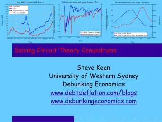
Solving Circuit Theory Conundrums. Steve Keen University of Western Sydney Debunking Economics www.debtdeflation.com/blogs www.debunkingeconomics.com. Circuit Theory Conundrums.

E N D
Solving Circuit Theory Conundrums Steve Keen University of Western Sydney Debunking Economics www.debtdeflation.com/blogs www.debunkingeconomics.com
Circuit Theory Conundrums • “If on the other hand, wage-earners decide to keep part of their savings in the form of liquid balances, firms will get back from the market less money than they have initially injected in it … firms will be unable to repay to the banks the whole of their debt.” (Graziani 1989) • “For the sake of simplicity, we exclude the payment of interest to the banks.” (Bellofiore et al, 2000) • “The existence of monetary profits … has always been a conundrum for theoreticians of the monetary circuit. If money is created from bank credit, how can we explain profits if firms borrow just enough to cover wages that are simply spent on consumption goods and returned to firms to extinguish their initial debt … In other words, how can M become M+?” (Rochon 2005)
Mathematical logic to the rescue... • Circuit conundrums result from “thinking in statics” • Financial cycle too complex to follow verbally • Even “stock-flow consistent” modelling not suitable • Solution is to think dynamically in continuous time • Consider flows set in motion by a loan • See what the flows tell you • Use appropriate mathematics to model • Problem with neoclassical economics not maths per se • But “teleological mathematics” • Work out what you want to believe • Torture common sense until you “prove” it • Appropriate maths is a system of differential equations...
Consider simplest possible pure credit economy • As in Graziani 1989 & 2003: • No Central Bank or fiat money • 3 sectors • Firms/Capitalists • Workers/Households • Bankers/Banks • Single loan of $L to Firm sector • Creates $L of debt and $L money simultaneously • Initiates several flows between accounts • Debt compounding • Loan and deposit interest payments • Wages • Consumption...
Mathematical logic to the rescue... • Develop model from the flows alone • Stocks (system states) derived from integrating flows $ transfer Accounting • Analysing the flows... Rates of change of accounts: • Accounts stable if “flows in” equal “flows out”:
Mathematical logic to the rescue... • So system can be stable if: • Not obviously onerous conditions... Exploring further: • A is the loan interest rate (rL) times Firm debt (FL) • B is the deposit interest rate (rD) times Firm savings (FD) • C is some rate per year (say w) times FD • D is the deposit interest rate on Worker savings (WD) • E is some consumption rate (say w) times Worker savings • F is some consumption rate (say b) Banker savings (BI) • Equilibrium values are:
Mathematical logic to the rescue... • Solved with symbolic algebra program: • Two key conditions: • All accounts are positive if • b > rL • and w > rD • Which means??? • If (for example)... • The (after inflation) interest rate on loans is 5%; • The interest rate on deposits is 1%; and • Bankers spend their account balance more often than once every 20 years; and • Workers spend theirs more often than once every century • Then the system can be stable
Common sense (and Marx) to the rescue... • It’s actually very simple: • Capitalist borrows $100 • Generates $400 (money turns over 4 times in a year) • Pays $300 in wages + inputs, keeps $100 in profit • Uses $5 to pay interest on $100 debt • Pockets $75 (M+-M) after paying debt down by $20 • Expressed in terms of time lags, conditions under which credit-financed business is profitable are quite broad • tStime lag from M to M+ (1/4th year standard setting) • tWtime lag in workers consumption (1/26th year) • tBtime lag in bankers consumption (1 year) • Positive bank balances (and hence incomes—shown later) for broad range of parameter values...
Conditions for positive bank balances over time • Wide range of valid values: Viable even if turnover period is 7-10 years • Bank balances are positive if: • Surplus generated in production • & workers consume • & bankers spend • Fairly basic conditions for positive profits, wages, etc...
Conditions for positive incomes over time • Banker gross income easy to calculate • Interest on outstanding debt per year = rL.FL • Worker gross income also easy • Wage flow per year = w.FD • But what is w? Back to Marx & Sraffa: • Workers share of surplus (1-s) • Divided by time lag in going from M to M+ (tS) • So w= (1-s)/tS • What about capitalist profits? • Capitalists share of surplus (s) • Divided by time lag in going from M to M+ (tS) • So Profits= FD.(1-s)/tS • Also derivable from Price times Quantity minus Wages
Common sense (and Marx) to the rescue... • A Simulation (click here for software)...
Conditions for positive incomes over time • Banker gross income = rL.FL • Worker gross income = FD.(1-s)/tS • Capitalist gross income = FD.s/tS • All positive so long as FD > 0. • System so far purely monetary • Presumes physical system producing net surplus • Easily linked with basic production system • Output = Labour times labour productivity • Labour = Wage flow/Wage • Wage set by “Phillips curve” • What about prices? • Derive from equilibrium conditions:
Basic financial and physical equilibrium conditions • In equilibrium, physical output Q = physical demand D • Physical Output Q = a.L • Where L = Wage flow/Wage • So • Equilibrium physical demand will be • Flow of monetary demand divided by Price level • D= (Wages+Profits)/Price • (net interest cancels out) • D =(FD.s/tS)/P • Equating D and Q: Cancel Cancel Cancel Cancel • Solve for P: • Surplusthe source of profit • Price converts capitalist share of surplus in production into monetary sum
Basic financial and physical equilibrium conditions • Dynamic price relation is • Time-lagged convergence to equilibrium value • Full monetary productionmodel can now be examined • Equilibrium conditions are (for given wage W): Simulation:
Common sense to the rescue... • Capitalists can therefore • borrow money; • pay interest; • repay debt; • & still make a profit • Aggregate profit exceeds zero • As do wages and interest income • Price converts capitalist surplus in production into money • M becomes M+ via the price mechanism • (if there is a surplus in production) • Fixed stock of money can finance constant output • Rising M not needed to sustain constant output
Common sense (and Marx) to the rescue... • Contrary Circuit conclusions resulted from • Confusion of stocks & flows: • Initial Loan (stock) is not the limit of financial transactions the money it creates can cause (Flow/Year) • Forgetting about surplus in production • Source of both physical and financial profit • Forgetting about turnover period of capital: • “Let the period of turnover be 5 weeks, : the working period 4 weeks... In a year of 50 weeks ... Capital I of £2,000, constantly employed in the working period, is therefore turned over 12½ times. 12½ times 2,000 makes £25,000.” (Capital II, Part II: The Turnover of Capital)
A new approach to dynamic modelling • Inspired by Godley/Lavoie Stock-Flow Consistent tables • Plus comments by Scott Fullwiler at UMKC 2006 • Rendition of SAM tabular concept in continuous time • With bank account fundamental unit of analysis • Far more suitable for asynchronous real-world • All investment does not occur at same time • Discrete “t”, “t-1” period modelling imposes this • Does not require artificial time-delays • Allows processes to occur at different frequencies • Consumption fortnightly, investment 2-yearly • See my Rossi-Ponsot 2009 chapter for more details • Easily implemented in any symbolic algebra program • (Mathcad—www.ptc.com/mathcad—shown here...)
A new approach to dynamic modelling • Input table of accounts and flows between them: $ transfer Accounting • Substitute functions for placeholders A, B, etc.: • Automatically build “coupled ODE” model
Conclusion: The Circuit “Works” • Long-believed conundrums must be forgotten... But • Solving conundrums strengthens Circuit Theory • Can explain where monetary profit comes from • System stable in the absence of Ponzi finance! • Model expands to growth, multiple sectors, fiat money • Explains: • Endogenous credit money creation; • Credit system’s desire to extend too credit; • Bank surplus rises if Debt rises • Basis of “inherent instability” in Financial Instability Theorem • Not just a Hypothesis! • Model here merely start of modelling monetary dynamics...
The Circuit can be extended... • To general monetary dynamic disequilibrium model... • Mixed credit-fiat money... • Comparing different policies