Phylogenetic Trees (2) Lecture 12
370 likes | 740 Vues
Phylogenetic Trees (2) Lecture 12. Based on: Durbin et al Section 7.3, 7.8, Gusfield: Algorithms on Strings, Trees, and Sequences Section 17. Recall: The Four Points Condition. Theorem: A set M of L objects is additive iff any subset of four objects can be labeled i,j,k,l so that:

Phylogenetic Trees (2) Lecture 12
E N D
Presentation Transcript
Phylogenetic Trees (2)Lecture 12 Based on: Durbin et al Section 7.3, 7.8, Gusfield: Algorithms on Strings, Trees, and Sequences Section 17. .
Recall: The Four Points Condition Theorem: A set M of L objectsis additive iff any subset of four objects can be labeled i,j,k,l so that: d(i,k) + d(j,l) = d(i,l) +d(k,j) ≥ d(i,j) + d(k,l) We call {{i,j},{k,l}} the “split” of {i,j,k,l}. The four point condition doesn’t provides an algorithm to construct a tree from distance matrix, or to decide that there is no such tree (ie, that the set is not additive). The first methods for constructing trees for additive sets used neighbor joining methods:
Constructing additive trees:The neighbor joining problem • Let i, j be neighboring leaves in a tree, let k be their parent, and let m be any other vertex. • The formula • shows that we can compute the distances of k to all other leaves. This suggest the following method to construct tree from a distance matrix: • Find neighboring leaves i,j in the tree, • Replace i,j by their parent k and recursively construct a tree T for the smaller set. • Add i,j as children of k in T.
A B C D Neighbor Finding How can we find from distances alone a pair of nodes which are neighboring leaves (called “cherries”)? Closest nodes aren’t necessarily cherries. Next we show one way to find neighbors from distances.
Neighbor Finding: Seitou&Nei method (87) Definitions Theorem (Saitou&Nei)Assume all edge weights are positive. If D(i,j) is minimal (among all pairs of leaves), then i and j are neighboring leaves in the tree.
Saitou&Nei proof Definitions path(i,j) = the path from leaf i to leaf j; d(u,path(i,j)) = distance in T from u to path(i,j). u d(u,path(i,j)) path(i,j) i j
Saitou&Nei proof ri rj -2d(u,path(i,j))
Rest of T u e i j Seitou&Nei proof For a vertex i, and an edge e=(i’,j’): Ni(e) = |{u : e is on path(i,u)}| Then: Note: If e is adjacent to a leaf, then w(e) is added exactly once to Q(i,j).
Saitou&Nei proof Assume for contradiction that Q(i,j) is maximized for i,j which are not neighboring leaves. Let path(i,j) = (i,,...,k,j), T1 be the subtree rooted at k, and assume WLOGthatT1has at most L/2 leaves. T2 = T \ T1. Let i’,j’ be any two neighboring leaves in T1. We will show that Q(i’,j’) > Q(i,j). T2 i’ j’ T1 j i k
Saitou&Nei proof Proof that Q(i’,j’)>Q(i,j): i’ T2 j’ T1 j i k Each leaf edgee adds w(e) both to Q(i,j) and to Q(i’,j’), so we can ignore the contribution of leaf edges to both Q(i,j) and Q(i’,j’)
Saitou&Nei proof Contribution of internal edges to Q(i,j) and to Q(i’,j’) i’ T2 j’ T1 j i k Since there is at least one internal edge e in path(i,j), Q(i’,j’) > Q(i,j). QED
A simpler neighbor finding method: Select an arbitrary node r. r d(r,path(i,j)) j Claim (from final exam, Winter 02-3): Let i, j be such that d(r,path(i,j))is maximized. Then i and j are neighboring leaves. i
r k i j Neighbor Joining Algorithm • If L =3, return tree of three vertices • Set M to contain all leaves, and select a root r. • Compute for all i,j ≠ r, C(i,j)=(d(r,i)+d(r,j)-d(i,j))/2. Iteration: • Choose i,j such that C(i,j) is maximal • Create new vertex k, and set C(i,j) • remove i,j, and add k to M • Recursively construct a tree on the smaller set, then add i,j as children on k, at distances d(i,k) and d(j,k).
Complexity of Neighbor Joining Algorithm (using the simpler neighbor finding method) Naive Implementation: Initialization:θ(L2) to compute d(r,i) and C(i,j) for all i,jL. Each Iteration: • O(L2) to find the maximal C(i,j). • O(L) to compute {C(m,k):m L} for the new node k. Total of O(L3). r C(m,k) m k
Complexity of Neighbor Joining Algorithm Using Heap to store the C(i,j)’s: Input: d(i,j) for all i,j, and an arbitrary vertex r. Initialization:θ(L2) to compute and heapify the C(i,j)’s. Each Iteration: • O(log L) to find and delete the maximal C(i,j). • O(1) to delete {d(r,i), d(r,j)} and add d(r,k). • O(L) to and update d(k,m) for all vertices m • O(L logL) to delete {C(i,m), C(j,m)} and add C(k,m) for all vertices m. Total of O(L2log L). (implementation details are omitted)
Ultrametric trees Definition:An ultrametric tree is a rooted weighted tree all of whose leaves are at the same depth. Basic property: Define the height of the leaves to be 0. Then edge weights can be represented by the heights of internal vertices. 8 3 5 Edge weights: 5 2 3 Internal-vertices heights: 5 3 3 3 3 3 0: A E D B C
8 5 3 3 A E D B C Least Common Ancestor and distances in Ultrametric Tree Let LCA(i,j) denote the least common ancestor of leaves i and j. Let height(LCA(i, j)) be its distance from the leaves, and dist(i,j) be the distance from i to j. Observation: For any pair of leaves i, j in an ultrametric tree: height(LCA(i,j)) = 0.5 dist(i,j).
Ultrametric Matrices Definition: A distances matrix* U of dimension LL is ultrametric iff for each 3 indices i, j, k : U(i,j) ≤ max {U(i,k),U(j,k)}. Theorem: The following conditions are equivalent for an LL distance matrix U: • U is an ultrametric matrix. • There is an ultrametric tree with L leaves such that for each pair of leaves i,j: U(i,j) = height(LCA(i,j)) = ½ dist(i,j). * “distance matrix” is a symmetric matrix with positive non-diagonal entries, 0 diagonal entries, which satisfies the triangle inequality.
Ultrametric tree Ultrametric matrix There is an ultrametric tree s.t. U(i,j)=½dist(i,j). U is an ultrametric matrix: By properties of Least Common Ancestors in trees U(k,i) = U(j,i) ≥U(k,j) i j k
Observations needed for proving Ultrametric matrix Ultrametric tree: Definition: Let U be an LL matrix, and let S {1,...,L}. U[S] is the submatrix of U consisting of the rows and columns with indices from S. Observation 1: U is ultrametric iff for every S {1,...,L}, U[S] is ultrametric. Observation 2: If U is ultrametric and maxi,jU(i,j)=m, , then m appears in every row of U. One of the “?” Must be m
9 i j Ultrametric matrix Ultrametric tree:Proof by induction U is an ultrametric matrix U has an ultrametric tree : By induction on L, the size of U. Basis: L= 1: T is a leaf L= 2: T is a tree with two leaves i i i i j i j
Induction step Induction step: L>2. Use the 1st row to split the set {1,…,L} to two subsets: S1 ={i: U(1,i) =m}, S2={1,..,L}-S (note: 0<|Si|<L) S1={2,4}, S2={1,3,5}
m=m1 m - m2 m2< m T1 T2 Induction step By Observation 1, U[S1] and U[S2] are ultrametric. By induction, tree T1 for S1, rooted at m1≤ m, and a tree T2 for S2 with root labeled m2 < m(m2 is the 2nd largest element in row 1; if m2=0 then T2 is a leaf). Join T1 and T2 to T with a root labeled m. [The construction when m1 = m]
m=m2 m1 T2 T1 Correctness Proof Need to prove: T is an ultrametric tree for U ie, U(i,j) is the label of the LCA of i and j in T. If i and j are in the same subtree, this holds by induction. Else LCA(i,j) = m (since they are in different subtrees). Also, [U(1,i)= m and U(1,j) ≠ m] U(i,j) = m.
Complexity Analysis Let f(L) be the time complexity for L×L matrix. f(1) ≤ f(2) = constant. For L>2: • Constructing S1 and S2: O(L). Let |S1| = k, |S2| = L-k. • Constructing T1 and T2: f(k)+f(L-k). • Joining T1 and T2 to T: Constant. Thus we have: f(L) ≤ maxk[ f(k) + f(L-k)] +cL, 0 < k < L. f(L) = cL2satisfies the above. Need an appropriate data structure! Thecondition U(i,j) ≤ max {U(i,k),U(j,k)} is easier to check than the 4 points condition. Therefore the theorem implies that ultrametric additive sets are easier to characterize then arbitrary additive sets.
8 3 5 B 3 C D A E Additive trees via Ultrametric trees Recent (and more efficient) ways for constructing and identifying additive trees use ultrametric trees. Idea: Reduce the problem to constructing trees by the “heights” of the internal nodes. For leaves i,j, U(i,j) represent the “height” of the common ancestor of i and j.
Transforming Weighted Trees to Ultrametric Trees First we set the height of all leaves to 0, by transforming the weighted Tree T to an ultrametric tree T’ as follows: Step 1: Pick a node k as a root, and “hang” the tree at k. a c a 2 k=a 2 4 1 3 3 b 2 1 b d 2 4 c d
Transforming Weighted Trees to Ultrametric Trees Step 2: Let M = maxid(i,k). M is taken to be the height of T’. Label the root by M, and label each internal node j by M-d(k,j). 9 a c a 2 k=a, M=9 7 2 4 1 3 3 2 b 4 1 2 d b 4 d c
9 2 7 9 3 7 4 4 4 a b c d Transforming Weighted Trees to Ultrametric Trees Step 3 (and last): “Stretch” edges of leaves so that they are all at distance M from the root 9 (9) a 2 7 M=9 1 3 (6) b 4 2 4 d (2) c (0)
9 2 7 9 (-9) 3 7(-6) 4 4 4(-2) a b c d Reconstructing the Weighted Tree from the Ultrametric Tree Weight of an internal edge is the difference between its endpoints. Weights of an edge to leaf i is obtained by substracting M-d(k,i) from its current weight. 2 0 a 1 3 b 4 2 c d M = 9
Solving the Additive Tree Problem by the Ultrametric Problem: Outline • We solve the additive tree problem by reducing it to the ultrametric problem as follows: • Given an input matrix D = D(i,j) of distances, transform it to a matrix U= U(i,j), where U(i,j) is the height of the LCA of i and j in the corresponding ultrametric tree TU. • Construct the ultrametric tree, TU, for U. • Reconstruct the additive tree T from TU.
How U is constructed from D U(i,j) should be the height of the Least Common Ancestror of i and j in TU, the ultrametric tree hanged at k: Thus, U(i,j) = M - d(k,m), where d(k,m) is computed by: 9 a 2 7 1 3 For k=a, i=b, j=c, we have: U(b,c)=9 - ½(3+9-8)=7 b 2 4 c d
a 2 1 3 b 2 4 d c The transformation D UTUT M=9 9 TU T 7 4 b a c d U D