MICE RF Cavity Measurements
130 likes | 269 Vues
MICE RF Cavity Measurements. Derun Li Center for Beam Physics Lawrence Berkeley National Laboratory March 26, 2010 University of California, Riverside, California. Summary. What we have so far The first five MICE RF cavity bodies arrived LBNL in December 2009

MICE RF Cavity Measurements
E N D
Presentation Transcript
MICE RF Cavity Measurements Derun Li Center for Beam Physics Lawrence Berkeley National Laboratory March 26, 2010 University of California, Riverside, California
Summary • What we have so far • The first five MICE RF cavity bodies arrived LBNL in December 2009 • Three completed Be windows at LBNL • CMM and low power RF measurements • Design and construction for lifting fixture • Design and construction of stands for RF measurements • Extension for CMM measurements • RF Measurement results of two MICE cavities • Preliminary analysis • Near term plans MICE RF Cavity Measurements, D. Li, Lawrence Berkeley National Lab, 3/26/2010
The RF Cavity at LBNL MICE RF Cavity Measurements, D. Li, Lawrence Berkeley National Lab, 3/26/2010
CMM Scans of MICE Cavity • Special probe to measure the inside profile of the cavity • Cavity interior profile being measured with special probe • ( 1,800 points per scan) • The profile will be used to verify cavity RF models MICE RF Cavity Measurements, D. Li, Lawrence Berkeley National Lab, 3/26/2010
Preparation for RF measurements Lifting fixtures Stand for RF measurements MICE RF Cavity Measurements, D. Li, Lawrence Berkeley National Lab, 3/26/2010
RF measurements, Team Work! Be window installation MICE RF Cavity Measurements, D. Li, Lawrence Berkeley National Lab, 3/26/2010
RF Measurements, Results S11 measurements S21 measurements MICE RF Cavity Measurements, D. Li, Lawrence Berkeley National Lab, 3/26/2010
MICE Cavity Design Parameters • The cavity design parameters • Frequency: 201.25 MHz • β = 0.87 • Shunt impedance (VT2/P): ~ 22 MΩ/m • Quality factor (Q0): ~ 53,500 • Be window diameter and thickness: 42-cm and 0.38-mm • Nominal parameters for MICE and cooling channels in a neutrino factory • 8 MV/m (~16 MV/m) peak accelerating field • Peak input RF power: 1 MW (~4.6 MW) per cavity • Average power dissipation per cavity: 1 kW (~8.4 kW) • Average power dissipation per Be window: 12 watts (~100 watts) MICE RF Cavity Measurements, D. Li, Lawrence Berkeley National Lab, 3/26/2010
Measurement Results • Two cavities have been measured in different window configurations using Be windows #1 and #2 • MICE cavity #1: S21 measurements (2 probes) with all ports shorted: Q 44,000 – 44, 600 (over 80% of the design Q) • MICE cavity #4: S21 measurements (2 probes) with all ports shorted: Q 43,600 – 44, 000 (over 80% of the design Q) MICE RF Cavity Measurements, D. Li, Lawrence Berkeley National Lab, 3/26/2010
Measurements and Analysis • Measurements of frequency changes from RF ports • From open to short: +11 kHz/port (S11 measurements) • Preliminary analysis (S. Virostek) • Assuming there is a cavity body frequency (equivalent to the iris terminated by flat metal sheet/window), fbody • The curved Be window introduces frequency shifts of +Δf1 (out) by window #1 and - Δf2(in) by window #2 if neglecting 2nd order frequency shifts due to local field changes by the curved window, therefore: Measured frequency ≈ fbody± Δf1 ± Δf2 • The “±” depends on Be window configurations MICE RF Cavity Measurements, D. Li, Lawrence Berkeley National Lab, 3/26/2010
Measurement Data Analysis -Δf1 Window # 1 Cavity body frequency:fbody Window # 2 + Δf2 MICE RF Cavity Measurements, D. Li, Lawrence Berkeley National Lab, 3/26/2010
Data Analysis (cont’d) • Three measurements should determine fbody, Δf1 andΔf2 • From MICE cavity #1 measurements: 200.990 =fbody – Δf1 + Δf2 fbody = 201.084 MHz 199.786 = fbody – Δf1 – Δf2Δf1 = 0.697 MHz 201.179 = fbody + Δf1 – Δf2 Δf2 = 0.602 MHz • From MICE cavity #4 measurements: 200.642 =fbody – Δf1 + Δf2 fbody = 200.741 MHz 199.454 = fbody – Δf1 – Δf2Δf1 = 0.693 MHz 200.839 = fbody + Δf1 – Δf2 Δf2 = 0.594 MHz • Conclusions: • Profiles of the two windows must be different ( 100 kHz) • Cavity frequency variation within ± 400 kHz (prediction) • Be windows can be used as additional tuning knobs MICE RF Cavity Measurements, D. Li, Lawrence Berkeley National Lab, 3/26/2010
Near Term Plans • Physical measurements of the first five MICE cavities and threeBe windows • CMM scans • RF measurements of the remaining three MICE cavities • Find center (average) frequency of all (10) MICE cavities • Cavity tuning to the center frequency in combination with Be windows • Each cavity and Be window will be measured and labeled (identified) with fbody and Δf • Cavity coupler and tuner fabrication and tests (A. DeMello) MICE RF Cavity Measurements, D. Li, Lawrence Berkeley National Lab, 3/26/2010