Download
1 / 76
760 likes | 956 Vues
Simulation of emission tomography. Robert L. Harrison University of Washington Medical Center Seattle, Washington, USA Supported in part by PHS grants CA42593 and CA126593. What is emission tomography?. Nuclear Medicine. Radiotherapy. Radiology. (www.imaginis.com). (Stieber et al).

E N D
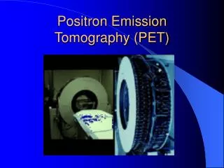
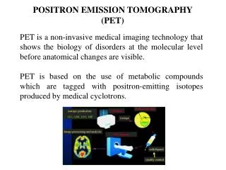
Simulation of emission tomography Robert L. Harrison University of Washington Medical Center Seattle, Washington, USA Supported in part by PHS grants CA42593 and CA126593
What is emission tomography? Nuclear Medicine Radiotherapy Radiology (www.imaginis.com) (Stieber et al) (Wikipedia)
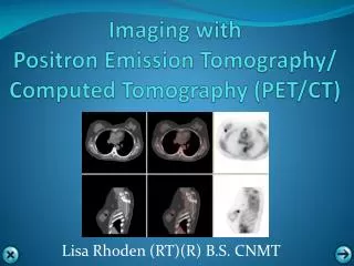
The difference between transmission and emission PET Positron emission tomography X-ray CT X-ray computed tomography Radiology Nuclear Medicine Unclear Medicine (Wikipedia)
Different information X-ray CT X-ray computed tomography PET Positron emission tomography PET/CT Anatomy/ Form Metabolism/ Function Complementary Information (Wikipedia)
Different information What’s the diagnosis? Dead…
Emission tomography:what should we simulate? Digital phantom Patient (Segars)
Emission tomography:what should we simulate? PET scanner Half scanners with and without collimation (Suetens) SPECT scanner Single photon emission computed tomography (George et al)
Emission tomography:what should we simulate? Signal processing / output event position
An example: SimSET A Simulation System for Emission Tomography • Goals - Flexible - Extensible - Portable - Easy-to-use - FAST
Object: voxelized • Voxelized objects: • Easier to define complex objects. • Patient scans are voxelized. • Faster tracking in complex objects. • Obvious which the next voxel is. • However, the time tracking through the object does increase as the voxelization grows finer.
Object: processes • Generate decays. • Decay products. • Tracking particles/photons. • Compton scatter. • Coherent scatter. • Photoabsorption. • Pair production. • Fluorescence. • Brehmstrahlung.
Object: generate next decay • Which voxel? Two options:
Object: generate next decay • Choose a random location in the voxel. How? - 3 random numbers, one each for x, y, z.
Object: generate next decay • When? • The mean number of decays in a voxel is the product of the scan time and the activity in the voxel. • The distribution of the actual number of decays is Poisson. • What distribution do we use to determine the elapsed time to the next decay? • The exponential distribution (1 random number). • Keep generating decays until the sum of the elapsed times is ≥ the scan time.
Object: generate next decay • What now? • Depends on the isotope: some combination of • alpha (Helium nuclei) • beta (electrons or positrons) • gamma (photons) • SimSET only produces one particle per decay: • positron (PET); or • photon (SPECT) < 1000 keV, all photons one energy. • No 124I, a positron emitter that also emits photons:
Object: annihilate positron (PET only) • SimSET does not track positrons. • Too many interactions; too computationally intensive. • Uses a probabilistic range model instead. • Positron/electron annihilation at end of range. • Two (almost) anti-parallel 511 keV photons produced. • Photon polarization not modeled.
Object: pick photon direction • Generate a random 3D unit vector. How? • 2 random numbers: • One picks an azimuthal angle between 0 and . • The other picks the cosine of the inclination angle between -1 and 1. • This results in a uniform distribution over the unit sphere.
Object: track photons • How far will a photon travel in a uniform medium? • is the material’s attenuation coefficient.
Object: track photons • How far will a photon travel in a changing medium? • Sample a dimensionless distance, free paths, p, from the exponential distribution with = 1. • Weight the distance traveled by the true ’s. Travel until dii = p
Object: photon interaction • If the photon leaves the object before traveling the sampled number of free paths, we pass it to the collimator module. • Otherwise randomly choose an interaction from: • Photoabsorption. • Compton scatter. • Coherent scatter. • If the photon scatters, continue tracking. • SimSET does not model pair production or secondary photons.
Object: choosing interaction type • If the probability of: • Photoabsorption is p < 1; • Compton scatter is c < 1 - p; • Coherent scatter is 1 - p - c. • Sample u randomly from (0,1). • If u < p then photoabsorb; p < u < p + c then Compton scatter; u ≥ p + c then coherent scatter.
Object: simulating interactions • Photoabsorption: • Discard photon. • Compton scatter: • Klein-Nishini density function to determine the scatter angle. • Acceptance-rejection method. • Klein-Nishina is a free electron approximation. • Photon loses energy as function of scatter angle. • Coherent scatter: • Table lookup with linear interpolation to determine scatter angle. • No energy lost. • Generally very small angles (< 5 degrees).
Collimators • Tracking is the same as through object. • Fluorescence (ignored in SimSET) is an issue for Thallium SPECT and deadtime. • Efficiency is a problem. Of decays in the FOV, • PET: only 1/20 - 1/200 detected. • SPECT: only 1/10000 - 1/1000000 are detected.
Collimators • SPECT collimators • Hunk of lead with hexagonal holes. • Collimator and detector circle patient. • SimSET models geometric collimator. • PET collimators • Cylindrical annuli of lead or tungsten to reduce randoms and scatter. • Trend towards no collimation in FOV.
Collimators • SimSET models only the collimators shown on previous slide. • Other collimation possibilities (mainly SPECT): • Pinhole. • Rotating slat. • Slit. • Electronic. • When (if) the photon escapes the collimator, SimSET passes it to the detector module.
Detectors • Tracking remains the same, but our interests change. • We are now interested in where/how much energy is deposited.
Detectors/electronics • When a photon interaction deposits energy in the detector crystal, the energy is converted into a shower of scintillation photons. • The photomultiplier tubes convert (some of) these photons into a electrical signals. • The electronics convert the signals into a detected position and energy. • Multiple interactions usually lead to incorrect positioning.
Detectors/electronics • SimSET ignores the scintillation photons. • These could be tracked. • Detected position is computed using the energy-weighted centroid of the interactions in crystal. • Detected energy is the sum of the energies deposited in crystal. It can be ‘blurred’ with a Gaussian. • For PET, time-of-flight offset is computed - it can be blurred as well.
Binning • Line-of-response or crystal pair. • Detected energy. • True, scatter, or random (PET only) state. • Time-of-flight position (PET only). (Schmitz)
Take away • For emission tomography, the patient is injected with (or ingests, etc.) a radio-labeled tracer. • Emission tomography is used to explore metabolism. • One type of simulation tracks individual photons through the ‘patient’, collimators and detectors. • Designing such a simulation requires knowledge of photon interactions with matter. • Some details may be skipped to improve efficiency, but this will bias the results and should be done with care.
References J.T. Bushberg, The essential physics of medical imaging, Lippincott Williams & Wilkins, 2002. K.P. George et al, Brain Imaging in Neurocommunicative Disorders, in Medical speech-language pathology: a practitioner's guide, ed. A.F. Johnson, Thieme, 1998. D.E. Heron et al, FDG-PET and PET/CT in Radiation Therapy Simulation and Management of Patients Who Have Primary and Recurrent Breast Cancer, PET Clin, 1:39–49, 2006. E.G.A. Aird and J. Conway, CT simulation for radiotherapy treatment planning, British J Radiology, 75:937-949, 2002. R. McGarry and A.T. Turrisi, Lung Cancer, in Handbook of Radiation Oncology: Basic Principles and Clinical Protocols, ed. B.G. Haffty and L.D. Wilson, Jones & Bartlett Publishers, 2008. R. Schmitz et al, The Physics of PET/CT Scanners, in PET and PET/CT: a clinical guide, ed. E. Lin and A. Alavi, Thieme, 2005. W.P. Segars and B.M.W. Tsui, Study of the efficacy of respiratory gating in myocardial SPECT using the new 4-D NCAT phantom, IEEE Transactions on Nuclear Science, 49(3):675-679, 2002. V.W. Stieber et al, Central Nervous System Tumors, in Technical Basis of Radiation Therapy: Practical Clinical Applications, ed. S.H. Levitt et al, Springer, 2008. P. Suetens, Fundamentals of medical imaging, Cambridge University Press, 2002. depts.washington.edu/simset/html/simset_main.html www.wofford.org/ecs/ScientificProgramming/MonteCarlo/index.htm www.impactscan.org/slides/impactcourse/introduction_to_ct_in_radiotherapy
What is SimSET used for? • Optimizing patient studies. • Assessing and improving quantitation. • Prototyping tomographs.
Variance reduction goal • Increase the precision of the simulation output achieved for a given effort: • Precision of the output is partly dependent on the number of detections. • Effort is the amount of CPU time we need for the simulation.
Variance reduction concepts • Increasing the efficiency of photon tracking. • Bias. • Data correlations. • Importance sampling. • Measuring efficiency.
Variance reduction concepts: photon tracking efficiency. • Decrease the amount of time we spend per photon OR • Increase the likelihood that each photon will be detected.
Variance reduction concepts: photon tracking efficiency. • In general, decreasing the time spent tracking a photon is considered code optimization (not variance reduction). • Most variance reduction methods increase the likelihood that photons will be detected. • In emission tomography only 1/20th (3D PET) to 1/100000th (SPECT) of decays are detected.
Variance reduction concepts: bias • Variance reduction methods can be unbiased or biased. • Unbiased methods are safer. • Biased methods can greatly increase apparent efficiency.
Variance reduction concepts: data correlations • In experimental data, different events are uncorrelated. • Many variance reduction methods add correlations between events. • In choosing variance reduction methods to use, be clear about how much correlation is acceptable.
Variance reduction concepts: importance sampling • We can create more decays in cone A than cone B, • but this would bias our output data. • To avoid bias we give each decay a weight that tells us how many ‘real world’ decays it represents. • For our output data we sum weights rather than incrementing counts. • In all variance reduction techniques, the weight of a decay/photon is adjusted to eliminate bias.
If we oversample cone A by a factor of 2, and undersample cone B by a factor of 10, we will collect a lot of events with weight 0.5. Variance reduction concepts: measuring efficiency
But occasionally an event from cone B will scatter and be detected with weight 10. Variance reduction concepts: measuring efficiency
Variance reduction concepts: measuring efficiency • A list of N non-uniformly weighted events is not as valuable as a list of N uniformly weighted events (e.g. counts). • How valuable are non-uniformly weighted events?