Download

1 / 28
280 likes | 546 Vues
Update to the GEO-CAPE Community and Working Group. Ken Pickering Project Scientist NASA GSFC Kenneth.E.Pickering@nasa.gov Gao Chen Data Manager NASA LaRC Gao.Chen@nasa.gov. Jim Crawford Principal Investigator NASA LaRC James.H.Crawford@nasa.gov Mary Kleb Project Manager NASA LaRC

E N D
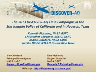
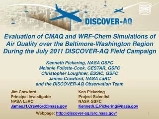
Update to the GEO-CAPE Community and Working Group Ken Pickering Project Scientist NASA GSFC Kenneth.E.Pickering@nasa.gov Gao Chen Data Manager NASA LaRC Gao.Chen@nasa.gov Jim Crawford Principal Investigator NASA LaRC James.H.Crawford@nasa.gov Mary Kleb Project Manager NASA LaRC Mary.M.Kleb@nasa.gov Website: http://discover-aq/larc.nasa.gov
Investigation Overview Deriving Information on Surface Conditions from Column and VERtically Resolved Observations Relevant to Air Quality A NASA Earth Venture campaign campaign intended to improve the interpretation of satellite observations to diagnose near-surface conditions relating to air quality Objectives: 1. Relate column observations to surface conditions for aerosols and key trace gases O3, NO2, and CH2O 2. Characterize differences in diurnal variation of surface and column observations for key trace gases and aerosols 3. Examine horizontal scales of variability affecting satellites and model calculations NASA UC-12 NASA P-3B Deployments and key collaborators Maryland, July 2011 (EPA, MDE, UMd, and Howard U.) California, January 2013 (EPA and CARB) Texas, September 2013 (EPA, TCEQ, and U. of Houston) TBD, Summer 2014 NATIVE, EPA AQS, and associated Ground sites
Deployment Strategy Systematic and concurrent observation of column-integrated, surface, and vertically-resolved distributions of aerosols and trace gases relevant to air quality as they evolve throughout the day. Three major observational components: NASA UC-12 (Remote sensing) Continuous mapping of aerosols with HSRL and trace gas columns with ACAM NASA P-3B (in situ meas.) In situ profiling of aerosols and trace gases over surface measurement sites Ground sites In situ trace gases and aerosols with AQS, NATIVE, and EPA Remote sensing of trace gas and aerosol columns with Pandora and Aeronet Ozonesondes Aerosol lidar observations
Baltimore-DC Flight Plan Plan as of 2/8/11 Green Line: UC-12 flight path Green Boxes: estimated ACAM swath Yellow Line: P-3B flight path Red line: R-4001 restricted area (cameras off during overflight) Blue Line: ICAO FIR Boundary
Additional Ground-Based Observations (Aeronet)
Additional Ground-Based Observations Trace Gas and aerosol measurements Fairhill: COMMIT Mobile Lab (Si CheeTsay and Can Li) Tethered Balloons (from surface to 1000 ft) Edgewood: Rich Clark (Millersville University) Beltsville: Everette Joseph (Howard University) and Jose Fuentes (Penn State) Remote Sensing Edgewood: LeosphereWindcube and Sigma Space MPL Beltsville: VaisalaCeilometer
Additional Airborne Observations University of Maryland (Russ Dickerson and Jeff Stehr) Regional Atmospheric Measurement Modeling and Prediction Program: http://www.atmos.umd.edu/~RAMMPP/ Cessna 402b In situ trace gas and aerosol payload - strong overlap with P-3B Flights have already begun Will provide valuable regional context to DISCOVER-AQ
Schedule SEAC4RS DC3 • Data archived and available to the public four months after each deployment • Pandora spectrometers will remain in place after each campaign deployment • Extended gap after first deployment offers an opportunity to improve the observational strategy for later deployments
DISCOVER-AQ Baltimore-Washington Field MissionForecasting for Flight Planning • Team: Ken Pickering, Melanie Follette-Cook, Bryan Duncan - NASA Clare Flynn, Chris Loughner - UMD, Greg Garner – PSU • Sources of forecast guidance: Meteorology: NCEP North American Mesoscale Model (NAM) UMD AOSC WRF NASA GEOS-5 (0.25 x 0.13 deg) NWS Sterling VA weather discussions; cloud forecasts Sterling, VA, Wakefield VA, Dover, DE radars Lidar-, ceilometer-, wind profiler-based boundary layer depths Air Quality: - NOAA operational CMAQ ozone and experimental PM2.5 forecast guidance (Pius Lee and Rick Saylor, NOAA/ARL) - CMAQ PM2.5 forecasts with NRT GOES fire emissions (Sundar Christopher, UAH) - NASA GEOS-5 on-line tracers [GOCART aerosols, CO, CO2, SO2] (Arlindo da Silva, NASA/GSFC)
Types of Flight Conditions: • A wide variety of cloud conditions ranging from clear to 50% partial cloudiness (fair weather Cu OK; avoid stratus decks) • A variety of ozone and PM conditions (moderate to severe pollution) • Light (near stagnation) to moderate wind speed conditions • A mix of local pollution and transport from upwind source regions (elevated pollution reservoir) • Chesapeake Bay breeze conditions • Before and after a thunderstorm passage • Sunrise (chemical evolution, low-level jet, subsequent BL growth)
Research and Analysis Activities • Statistical analysis – correlations between surface PM2.5 and AOD, surface and column NO2, O3, etc. Study extent to which boundary layer depth and mixing, humidity, emissions, and chemistry influence the correlation between surface and column observations. • Improvement of retrieval algorithms through insights obtained from the combination of ACAM, Pandora, aircraft, and surface data. Comparisons with MODIS, OMI, GOME-2, TES. Data available for testing GEO-CAPE algorithms. • Regional air quality modeling - WRF-Chem and CMAQ simulations (≤ 4 km horizontal resolution) will be evaluated using all available data from the field mission. Use model output to interpret observations. Compute scaling factors between surface and column values in model and compare with those derived from observations. Use transport feature information from the model to explain inconsistencies between surface and column observations. • Assess spatial and temporal variability of trace gases and aerosols in models and observations; important information for design of GEO-CAPE.
Overall Goals of Regional Modelingfor DISCOVER-AQ • Unravel the details of factors controlling column amount versus surface quantities for trace gases and aerosols - Evaluate WRF-Chem and CMAQ using all available observations from field mission - Compute scaling factors between surface and column values in model and compare with those derived from observations. - Use information concerning transport features from the model to explain inconsistencies between surface and column observations. - Use model output in spatial and temporal variability analyses in support of GEO-CAPE planning
Detailed List of Activities • Develop best possible set of emissions data for the study region from data sources such as CEMS, MARAMA, MDOT traffic counts, etc. • RACM2 (Bill Stockwell) chemical mechanism – will be in next CMAQ release. Need to get it into WRF-Chem also. • Evaluate WRF model boundary layer depths using sonde, lidar, aircraft, and ceilometer observations • Evaluation of chemical mechanisms and aerosol modules using surface, remotely sensed, and in-situ profile data. • How do scaling factors between surface and column quantities vary depending on boundary layer depth, transport, proximity to major sources, time of day, etc.
Detailed List of Activities • Examine spatial and temporal variations in surface and tropospheric column values in the models versus those derived from observations • Comparisons of model tropospheric column fields with satellite observations (OMI, GOME-2, MODIS, TES, etc.) • Fine-resolution (< 4 km) simulations to capture Chesapeake Bay Breeze
Weather Research & ForecastingModel (WRF) • Advanced Research WRF (ARW) core V3.2 • 32 levels in the vertical, up to 100 hPa • Initial and boundary conditions based on NARR (GEOS-5 possible) • Online Chemistry Module – V3.2 • CBMZ chemical mechanism and MOSAIC aerosol parameterization including some aqueous reactions 4 km 12 km 36 km • Initial and boundary conditions for trace gases and aerosols based on MOZART (NASA GMI possible) • Anthropogenic emissions generated by (Sparse Matrix Operator Kernel Emissions (SMOKE) modeling system using annual emissions from US Regional Planning Offices and hourly Contiguous Emissions Monitoring data from the EPA • Biogenic emissions from Biogenic Emissions Inventory System (BEIS) V3.12
MOSAIC 8-bin Aerosol Variables • 8 aerosol mass size bins* (μg/kg dry air): • SO4, NH4, NO3, Cl, Na, organic carbon, black carbon, other inorganics , water • 8 aerosol in cloud mass size bins* (μg/kg dry air): • SO4, NH4, NO3, Cl, Na, organic carbon, black carbon, and other inorganics • PM2.5 dry mass (μg/m3) • PM10 dry mass (μg/m3) • Backscatter coefficient • Single scattering albedo • Asymmetry parameter • Extinction coefficient • All at 4 wavelengths (300, 400, 600, and 999 nm) * Size bins range from 0.039 to 10 μm
Community Multiscale Air Quality Model (CMAQ) • Developed by EPA (Ching and Byun, 1999; Byun and Schere, 2006) • Applications: By state air quality agencies for regulatory modeling as part of State Implementation Plan process By EPA for national air quality assessments By NOAA for operational air quality forecast guidance • Current version: 4.7.1 (June 2010) Contains CB05 chemical mechanism; AE-5 aerosol module • WRF meteorological data processed by MCIP (Meteorology and Chemistry Interface Processor) • Emissions data sets developed using SMOKE
Trace Gas Species & Aerosols July 9, 2007 – 18 UTC Trop Column (sfc – 200 hPa) O3 NO2 CO SO2 HCHO PM2.5
WRF-Chem (12-km res.) vs. Beltsville, MD Ozonesonde Profiles Yegorova et al., JGR, subm., 2011
Trop. Column (sfc – 200 hPa) ACAM Column (sfc – 330 hPa) PBL Column Surface mixing ratio Sfc. O3 (ppbv) / Trop Col. O3 (1017 molec / cm2) Trop Column = sfc – 200 hPa
Loughner et al., 2011, Atmos. Environ, in press.WRF-UCM 2-m temperature and 10-m wind speed at 2000 UTC (3pm EST) July 9, 2007. A stronger temperature gradient along the coastline of the Chesapeake Bay in the 0.5km domain results in a stronger Bay breeze. 13.5km 0.5km
8-hr max O3 concentrations on July 9, 2007 from measurements and the base case simulation. Less pollutants over the water in the higher resolution simulations due to a stronger bay breeze results in lower ozone concentrations over the water. Convergence zone along western shore of bay leads to largest ozone values in that location Loughner et al., 2011, in press
CMAQ 1.5-km simulation Fair Hill * * Aldino * Edgewood * Essex
Spatial Variability in 4-km WRF-Chem Simulation 90% EV 75% 50% Follette-Cook et al., 2011, in prep.
Change in Variability During Daylight Hours Tropospheric Columns (sfc to 200 hPa) O3 NO2 Average Difference (1015molec/cm2) Average Difference (1017molec/cm2) Distance (km) 7 AM 9 AM 11 AM 1 PM 3 PM 5 PM EST
Collaborative Post-mission Modeling Activities • Pius Lee/Rick Saylor (NOAA/ARL) – Evaluation of operational CMAQ O3 forecasts and experimental PM2.5 forecasts • Maria Tzortziou (UMD/GSFC)– NASA New Investigator Program – Chesapeake Bay-focused research • Mian Chin (GSFC) – NASA Unified WRF containing GOCART aerosol • Arlindo da Silva (GSFC) – GEOS-5 GCM with GOCART aerosol and tracers • Ross Salawitch/Tim Canty (UMD) – MDE-sponsored CMAQ simulations • Russ Dickerson (UMD) – possible NASA AQAST activities • Xin-Zhang Liang (UMD) – black carbon studies using Climate-WRF More collaborators welcome!