Phylogenetic Trees (2) Lecture 13
Phylogenetic Trees (2) Lecture 13. Based on: Durbin et al 7.4, Gusfield 17.1-17.3, Setubal&Meidanis 6.1. Character-based methods for constructing phylogenies.

Phylogenetic Trees (2) Lecture 13
E N D
Presentation Transcript
Phylogenetic Trees (2)Lecture 13 Based on: Durbin et al 7.4, Gusfield 17.1-17.3, Setubal&Meidanis 6.1 .
Character-based methodsfor constructing phylogenies In this approach, trees are constructed by comparing the characters of the corresponding species. Characters may be morphological (teeth structures) or molecular (homologous DNA sequences). One common approach is Maximum Parsimony Common Assumptions: • Independence of characters (no interactions) • Best tree is one where minimal changes take place
Character based methods: Input data • Each character (column) is processed independently. • The green character will separate the human and pig from frog, horse and dog. • The red character will separate the dog and pig from frog, horse and human. • We seek for a tree that will best explain all characters simultaneously.
1. Maximum Parsimony A Character-based method Input: • h sequences (one per species), all of length k. Goal: • Find a tree with the input sequences at its leaves, and an assignment of sequences to internal nodes, such that the total number of changes is minimized.
AAA AAA AAA 2 1 1 GGA AGA AAG AAA Total #substitutions = 4 Example Input: four nucleotide sequences: AAG, AAA, GGA, AGA taken from four species. By the parsimony principle, we seek a tree that has a minimum total number of substitutions of symbols between species and their originator in the phylogenetic tree. Here is one possible tree
AAA AAA 1 AAA AAA AGA AAA 1 2 1 1 1 AAA AGA AGA GGA AAG GGA AAG AAA Total #substitutions = 3 Total #substitutions = 4 Example Continued There are many trees possible. For example: The left tree is preferred over the right tree. The total number of changes is called the parsimony score.
Example With One Letter Sequences • Suppose we have five species, such that three have ‘C’ and two ‘T’ at a specified position • Minimal tree has only one evolutionary change: C T C T C C C T T C
Aardvark Bison Chimp Dog Elephant Extension to Many Letters • What is the parsimony score of A: CAGGTA B: CAGACA C: CGGGTA D: TGCACT E: TGCGTA When the tree is known, we can do it character after character; each score is computed independently of the others.
Parsimony Based Reconstruction • Two separate components: • A procedure to find the minimum number of changes needed to explain the data (for a given tree topology, where species are assigned to leaves) • A search through the space of trees. • We will see that (1) is easy. (2) is hard.
A A/T Fitch Algorithm (Tree is Given) Work on each character independently. Start at the leaves. If two sisters have common character, parent “inherits” their intersection. Else, parent Inherits their union. After reaching root, go down to fix sets of size > 1. A A/C A T A A C
Fitch’s Algorithm, More Formally • traverse tree from leaves to root determining set of possible states (e.g. nucleotides) for each internal • node • traverse tree from root to leaves picking ancestral states for internal nodes
Fitch’s Algorithm – Phase 1 • do a post-order (from leaves to root) traversal of tree • Determine possible states Riof internal node i with children j and k
Fitch’s Algorithm – Phase 1 • # of changes = # of union operations TC C AGC CT GC C G T C A T
Fitch’s Algorithm – Phase 2 • do a pre-order (from root to leaves) traversal of tree • select state rj of internal node j with parenti as follows:
Fitch’s Algorithm – Phase 2 TC C AGC CT GC C G T C A T
Proof of Fitch’s Algorithm We’ll show that Fitch maximizes the parsimony score at every character. • Definitions: • For a leaf-labeled tree T, let T* be an optimal assignment of labels to internal nodes of T. • Let T*(v)be the assignment at internal node v under T*. • Let Tv be the tree rooted at v.
Claim: The first phase of Fitch keeps at v the set of states S(v) such that • For every s S(v), there exists an optimal tree Tv* with Tv*(v) = s, • In every optimal tree Tv* , Tv*(v) = s for some s S(v). • Proof: By induction of the tree height h. • Basis: h=1 • If both children have the same state – zero change. • Otherwise – exactly one change. A A B A A A B
Induction step: Assume correctness for height k and will prove for k+1. Let p1 and p2 be the optimal costs of the subtrees of v’s children. • If the intersection of v’s children lists is not empty, then the optimal score is p1+p2 and it can be achieved by labeling v with any member in the intersection, and only in this way. • Otherwise, the optimal score is p1+p2+1, and it can be achieved by labeling v with any member in the union of the lists, and only in this way. B A,B,C,D B,C C,D A,B A,B
Generalization: Weighted Parsimony(Sankoff’s algorithm) Weighted Parsimony score: • Each change is weighted by a score c(a,b). • The weighted parsimony score reduces to the parsimony score when c(a,a)=0 and c(a,b)=1 for all b other than a.
k j i Weighted Parsimony on a Given Tree Each position is independent and computed by itself. Use Dynamic programming on a given tree. • if k is a node with children i and j, then S(k,a) = minb(S(i,b)+c(a,b)) + minb’(S(j,b’)+c(a,b’)) S(j,b)the optimal score of a subtree rooted at j when j has the character b. S(k,a) S(i,b) S(j,b’)
Evaluating Parsimony Scores Dynamic programming on a given tree Initialization: • For each leaf i set S(i,a) = 0 if i is labeled by a, otherwise S(i,a) = Iteration: • if k is node with children i and j, then S(k,a) = minx(S(i,x)+c(a,x)) + miny(S(j,y)+c(a,y)) Termination: • cost of tree is minxS(r,x) where r is the root Comment: To reconstruct an optimal assignment, we need to keep in each node k and for each character a the two characters x, y that bring about the minimum when k has character a.
Cost of Evaluating Parsimony for binary trees If there are n nodes, m characters, and k possible values for each character, then complexity is O(nmk3). Of course, we still need to search over possible trees and find the best one. One usually resorts to heuristic search techniques.
2. The perfect phylogeny problem • A character is assumed to be a property which distinguishes between species (e.g. dental structure). • A characters state is a value of the character (human dental structure). • Problem: Given set of species, specified by their characters, reconstruct their evolutionary tree.
Homoplasy-free trees 1 Characters in Phylogenetic Trees should avoid:reversal transitions • A species regains a state it’s direct ancestor has lost. • Famous examples: • Teeth in birds. • Legs in snakes.
Homoplasy-free trees 2 …and also avoidconvergence transitions • Two species possess the same state while their least common ancestor possesses a different state. • Famous example: The marsupials.
Characters as Colorings A coloring of a tree T=(V,E) is a mapping C:V [set of colors] A partial coloring of T is a mapping defined on a subset of the vertices U V: C:U [set of colors] U=
Each character defines a (partial) coloring of the correspondeing phylogenetic tree: Characters as Colorings (2) Species ≡ VerticesStates ≡ Colors
Convex Colorings (and Characters) Let T=(V,E) be a colored tree, and d be a color. The d-carrier is the minimal subtree of T containing all vertices colored d Definition: A (partial/total) coloring of a tree is convex iff all d-carriers are disjoint C
Convexity Homoplasy Freedom A character is Homoplasy free (avoids reversal and convergence transitions) ↕ The corresponding (partial) coloring is convex
The Perfect Phylogeny Problem • Input: a set of species, and many characters, each assigns states (colors) to the species. • Question: is there a tree T containing the species as vertices, in which all the characters (colorings) are convex?
RRB BBR RRR RBR The Perfect Phylogeny Problem(pure graph theoretic setting) Input: Partial colorings (C1,…,Ck) of a set of vertices U (in the example: 3 total colorings: left, center, right, each by two colors). Problem: Is there a tree T=(V,E), s.t. UV and for i=1,…,k,, Ci is a convex (partial) coloring of T? NP-Hard In general, in P for some special cases
Perfect Phylogeny for a 0-1 Matrix Rows correspond to objects, columns to characters. Each character has two states: 0 (non exists) or 1 (exists). A tree T is a perfect phylogeny for the matrix iff it has the following properties: • Each of the n objects corresponds to a leaf of T. • Each of the m characters labels exactly one edge of T. • Object p has character ii labels an edge on thepath from p to the root. Note: [B and C hold] [each character is convex on T] C2 C3 C1 C4 E B D C5 A C
Perfect Phylogeny for a 0-1 Matrix By the definition, for each character C there is one edge in which it is converted from 0 to 1. In the below tree, the edge on which character C2 is converted to 1 is marked. The resulted tree is convex for this character. C2 E B D A C
C2 C3 C1 C4 E D B C5 A C The (Binary) Perfect Phylogeny Problem Problem: Given a 0-1 matrix M, determine if it has a perfect phylogeny, and construct one if it does. (Note: edges are labeled by characters: edge labeled by i represent changing character i’sstate from 0 to 1). As we show below, the answer is yes for our matrix:
Efficient algorithm for the Binary Perfect Phylogeny Problem Definition: Given a 0-1 matrix M, Ok={j:Mjk=1}, ie: Ok is the set of objects that have character Ck. Theorem: M has a perfect phylogenetic tree iff the sets {Oi} are laminar, ie: for all i, j, either Oi and Oj are disjoint, or one includes the other. Laminar Not Laminar
Proof : Assume M has a perfect phylogeny, and let i, j be given. Consider the edges labeled i and j. Case 1: There is a root to leaf path containing both. Then one is included in the other (2 and 1 below). Case 2: not case 1. Then they are disjoint (2 and 3 below). C2 C3 C1 C4 E D B C5 A C
C1 B A Proof (cont.) : Assume for all i, j, either Oi and Oj are disjoint, or one includes the other. We prove by induction on the number of characters that it has a perfect phylogenetic tree for the matrix. Basis: one character. Then there are at most two objects, one with and one without this character.
Proof (cont.) : Induction step: Assume correctness for n-1 characters, and consider a matrix with n characters (non-zero columns). WLOG assume that O1 is not contained in Oj for j > 1. Let S1 be the set of objects j for which Mj1= 1, and S2 be the remaining objects. Then each character belongs to objects in S1 or S2, but not both (prove!). By induction there are trees T1 andT2 for S1 and S2. Combining them as below gives the desired tree. 1 T1 T2