High-Pass Quantization for Mesh Encoding
High-Pass Quantization for Mesh Encoding. Olga Sorkine, Daniel Cohen-Or, Sivan Toledo Eurographics Symposium on Geometry Processing, Aachen 2003. Overview. Geometry quantization Visual quality Connection to spectral properties. Geometry quantization – introduction.


High-Pass Quantization for Mesh Encoding
E N D
Presentation Transcript
High-Pass Quantization for Mesh Encoding Olga Sorkine, Daniel Cohen-Or, Sivan Toledo Eurographics Symposium on Geometry Processing, Aachen 2003
Overview • Geometry quantization • Visual quality • Connection to spectral properties
Geometry quantization – introduction • Each mesh vertex is represented by Cartesian coordinates, in floating-point. • Geometry compression requires quantization, normally 10-16 bits/coordinate (xi, yi, zi)
Geometry quantization – introduction • Using smoothness assumptions, the quantized coordinates are predicted and the prediction errors are entropy-coded [Touma and Gotsman 98]
Quantization error • Quantization necessarily introduces errors. • The finer the sampling, the more it suffers.
Quantization error • An example: coarsely-sampled sphere original Quantized to 8 bits/coordinate
Quantization error • A finely-sampled sphere with the same quantization original Same quantization to 8 bits/coordinate
Quantization error – discussion • Quantization of the Cartesian coordinates introduces high-frequency errors to the surface. • High-frequency errors alter the visual appearance of the surface – affect normals and lighting. • Only conservative quantization (usually 12-16 bits) avoids these visual artifacts.
Quantization – our approach • Transform the Cartesian coordinates to another space using the Laplacian matrix of the mesh. • Quantize the transformed coordinates. • The quantization error in the regular Cartesian space will have low frequency. • Low-frequency errors are less apparent to a human observer.
Relative (laplacian) coordinates • Represent each vertex relatively to its neighbours average of the neighbours the relative coordinate vector
Laplacian matrix • A Matnn(R)the adjacency matrix • D Matnn(R) the degree-diagonal matrix: • Then, the Laplacian matrix L Matnn(R) is:
Laplacian matrix • The previous form is not symmetric. We will use the symmetric Laplacian:
Properties of L • Sort the eigenvalues of L in accending order: • We can represent the geometry in L’s eigenbasis: “frequencies” eigenvectors low frequency components high frequency components
Previous usages of Laplacian matrix • [Karni and Gotsman 00] – progressive geometry compression • Use the eigenvectors of L as a new basis of Rn • Transmit the coordinates according to this spectral basis • First transmit the lower-eigenvalue coefficients (low frequency components), then gradually add finer details by transmitting more coefficients.
Previous usages of Laplacian matrix • [Taubin 95] – surface smoothing • “Push” every vertex towards the centroid of its neighbours, i.e. • v’ = (I –L)v • Iterate, with positive and negative values of (to reduce shrinkage effect)
Previous usages of Laplacian matrix • [Ohbuchi et al. 01] – mesh watermarking • Embed a bitstring in the low-frequency coefficients • Changes in low-frequency components are not visible • [Alexa 02] – morphing using relative coordinates • Produces locally smoother morphs • [Gotsman et al. 03] • A more general class of Laplacian matrices • Mesh embedding on a sphere using eigenvectors
Quantizing the - coordinates • Transform Cartesian to -coordinates: • Quantize -coordinates • To get back Cartesian coordinates: (fixed-point quantization)
Discussion of the linear system • The matrix L is singular, so L1 doesn’t exist. • Adding one anchor point fixes this problem (substitute one vertex (x, y, z) – removes translation degrees of freedom)
Discussion of the linear system • By quantizing the , we put high-frequency error into . • L has very small eigenvalues, so L1 has very large eigenvalues ( 1/) • Thus, L1 amplifies small errors and reverses the frequencies. Small quantization error for , high frequency NOT so small !! low frequency
Spectrum of quantization error • Write x as: x=a1e1 + a2e2 + … + anen • Therefore, = Lx=1a1e1 + 2a2e2 + … + n-1an-1en-1+ nanen • Quantization error for ( + q ) is: q=c1e1 + c2e2 + … + cn-1en-1 + cnen • Resulting error in x: qx = L1 q=(1/1)c1e1 + (1/2)c2e2 + … + (1/n-1)cn-1en-1 + (1/n)cnen Small i – low frequencies large i – high frequencies low frequencies – small ci high frequency error – here ci are large (1/i) is small – attenuates high-frequency errors (1/i) is large – amplifies low-frequency errors Thus, the error in x will contain stronglow-frequency components but weak high-frequency components.
Discussion of the linear system • Example of low-frequency error: • Find the differences between the horses…
Discussion of the linear system • Example of low-frequency error: • This one is the original horse model
Discussion of the linear system • Example of low-frequency error: • This is the model after quantizing to 8 bits/coordinate • There is one anchor point (front left leg)
Making the error lower • We add moreanchor points, whose Cartesian coordinates are known, as well as the - coordinates. • This “nails” the geometry in place, reducing the low-frequency error
Rectangular Laplacian • We addequations for the anchor points • By adding anchors the matrix becomes rectangular, so we solve the system in least-squares sense: L constrained anchor points
Choosing the anchor points • A greedy scheme. • Add one anchor point at a time. • Each time nail down the vertex that achieved the maximal error after reconstruction. • This process is slow, but it is done only by the encoder. • Only a small number of anchors is needed. We experiment with 0.1%, which gives very good results.
The effect of anchors on the error Positive error – vertex moves outside of the surface 0 – Negative error – vertex moves inside the surface -quantization 7b/c 2 anchors -quantization 7b/c 4 anchors -quantization 7b/c 20 anchors Cartesian quantization 8b/c
Visual error metric • Euclidean distance between and does not faithfully represent the visual error (Cartesian quantization errors are small but the normals change a lot...) • Karni and Gotsman [2000] propose a “visual metric”: ║x – x’║vis = ║x – x’║2+(1 – )║GL(x) – GL(x’)║2 = 0.5 • We are not sure that should be 0.5…
Visual error metric • We measured the two error components separately: Mq= ║x – x’║2 Sq = ║GL(x) – GL(x’)║2 Evis = Mq+(1 – ) Sq
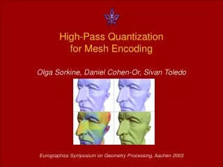
Some results We compare to Touma-Gotsman predictive coder that uses Cartesian quantization original -quantization, entropy 7.62 Cartesian quantization, entropy 7.64 Evis[=0.5] = 2.5 Evis[=0.15] = 2.6 Evis[=0.5] = 5.3 Evis[=0.15] = 2.3
Some results We compare to Touma-Gotsman predictive coder that uses Cartesian quantization original -quantization, entropy 6.69 Cartesian quantization, entropy 7.17 Evis[=0.5] = 1.8 Evis[=0.15] = 0.9 Evis[=0.5] = 4.8 Evis[=0.15] = 4.9
Some results We compare to Touma-Gotsman predictive coder that uses Cartesian quantization original -quantization, entropy 10.3 Cartesian quantization, entropy 10.3 Evis[=0.5] = 6.4 Evis[=0.15] = 3.9 Evis[=0.5] = 5.0 Evis[=0.15] = 5.1
Time statistics • The least-squares system was solved using QR factorization of the normal equations • Implementation on 2 GHz P4 using TAUCS library
Conclusions • The spectrum of the quantization error affects the visual quality of the quantized mesh • We have proposed a quantization method that concentrates the error in the low-frequencies • The method requires the computational effort of solving a linear least-squares system. • Much more research is needed to fully understand the spectral behavior of meshes…
Acknowledgements • Christian Rössl and Jens Vorsatz from Max-Planck-Institut für Informatik for the models • Israel Science Foundation founded by the Israel Academy of Sciences and Humanities • The Israeli Ministry of Science • IBM Faculty Partnership Award • German Israel Foundation (GIF) • EU research project ‘Multiresolution in Geometric Modelling (MINGLE)’, grant HPRN-CT-1999-00117.