Earley’s Algorithm (1970)
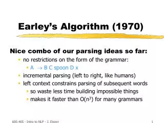
Earley’s Algorithm (1970). Nice combo of our parsing ideas so far: no restrictions on the form of the grammar: A B C spoon D x incremental parsing (left to right, like humans) left context constrains parsing of subsequent words so waste less time building impossible things

Earley’s Algorithm (1970)
E N D
Presentation Transcript
Earley’s Algorithm (1970) Nice combo of our parsing ideas so far: • no restrictions on the form of the grammar: • A B C spoon D x • incremental parsing (left to right, like humans) • left context constrains parsing of subsequent words • so waste less time building impossible things • makes it faster than O(n3) for many grammars 600.465 - Intro to NLP - J. Eisner
… … 600.465 - Intro to NLP - J. Eisner
A A D + = j k B C D E B C D E j i k i A B C . D E A B C D . E Overview of Earley’s Algorithm • Finds constituents and partial constituents in input • A B C . D E is partial: only the first half of the A 600.465 - Intro to NLP - J. Eisner
Overview of Earley’s Algorithm • Proceeds incrementally, left-to-right • Before it reads word 5, it has already built all hypotheses that are consistent with first 4 words • Reads word 5 & attaches it to immediately preceding hypotheses. Might yield new constituents that are then attached to hypotheses immediately preceding them … • E.g., attaching D to A B C . D E gives A B C D . E • Attaching E to that gives A B C D E . • Now we have a complete A that we can attach to hypotheses immediately preceding the A, etc. 600.465 - Intro to NLP - J. Eisner
Our Usual Example Grammar ROOT S S NP VP NP Papa NP Det N N caviar NP NP PP N spoon VP VP PP V ate VP V NP P with PP P NP Det the Det a 600.465 - Intro to NLP - J. Eisner
0 Papa 1 ate 2 the 3 caviar 4 with 5 a 6 spoon 7 First Try: Recursive Descent ROOT S VP VP PP NP Papa V ate S NP VP VP V NP N caviar P with NP Det N PP P NP N spoon Det the NP NP PP Det a • 0 ROOT . S 0 • 0 S . NP VP 0 • 0 NP . Papa 0 • 0 NP Papa . 1 • 0 S NP . VP 1 • 1 VP . VP PP 1 • 1 VP . VP PP 1 • 1 VP . VP PP 1 1 VP . VP PP 1 oops, stack overflowed • OK, let’s pretend that didn’t happen. • Let’s suppose we didn’t see VP VP PP, and used VP V NP instead. “goal stack” 600.465 - Intro to NLP - J. Eisner
0 Papa 1 ate 2 the 3 caviar 4 with 5 a 6 spoon 7 First Try: Recursive Descent ROOT S VP V NP NP Papa V ate S NP VP VP VP PP N caviar P with NP Det N PP P NP N spoon Det the NP NP PP Det a • 1VP . V NP 1after dot = nonterminal, so recursively look for it (“predict”) • 1V . ate 1after dot = terminal, so look for it in the input (“scan”) • 1 V ate . 2after dot = nothing, so parent’s subgoal is completed (“attach”) • 1 VP V . NP 2 predict (next subgoal) • 2NP . ... 2do some more parsing and eventually ... • 2NP ... . 7we complete the parent’s NP subgoal, so attach • 1 VP V NP .7 attach again • 0 S NP VP .7 attach again • 0 ROOT . S 0 • 0 S . NP VP 0 • 0 NP . Papa 0 • 0 NP Papa . 1 • 0 S NP . VP 1 after dot = nonterminal, so recursively look for it (“predict”) 600.465 - Intro to NLP - J. Eisner
0 Papa 1 ate 2 the 3 caviar 4 with 5 a 6 spoon 7 First Try: Recursive Descent ROOT S VP V NP NP Papa V ate S NP VP VP VP PP N caviar P with NP Det N PP P NP N spoon Det the NP NP PP Det a • 0 ROOT . S 0 • 0 S . NP VP 0 • 0 NP . Papa 0 • 0 NP Papa . 1 • 0 S NP . VP 1 • 1VP . V NP 1 • 1V . ate 1 • 1 V ate . 2 • 1 VP V . NP 2 • 2NP . ... 2 • 2NP ... . 7 • 1 VP V NP .7 • 0 S NP VP .7 implement by function calls: S() calls NP() and VP(), which recurse must backtrack to try predicting a different VP rule here instead But how about the other parse? 600.465 - Intro to NLP - J. Eisner
0 Papa 1 ate 2 the 3 caviar 4 with 5 a 6 spoon 7 First Try: Recursive Descent ROOT S VP V NP NP Papa V ate S NP VP VP VP PP N caviar P with NP Det N PP P NP N spoon Det the NP NP PP Det a • 1VP . V NP 1 • 1 V . ate 1 • 1 V ate . 2 • 1 VP V . NP 2 • 2NP . ... 2do some more parsing and eventually ... • 2NP ... . 4... the correct NP is from 2 to 4 this time (but might we find the one from 2 to 7 instead?) • 0 ROOT . S 0 • 0 S . NP VP 0 • 0 NP . Papa 0 • 0 NP Papa . 1 • 0 S NP . VP 1 • 1VP . VP PP 1 we’d better backtrack here too! (why?) 600.465 - Intro to NLP - J. Eisner
0 Papa 1 ate 2 the 3 caviar 4 with 5 a 6 spoon 7 First Try: Recursive Descent ROOT S VP V NP NP Papa V ate S NP VP VP VP PP N caviar P with NP Det N PP P NP N spoon Det the NP NP PP Det a • 1VP . VP PP 1 1VP . VP PP 1 1VP . VP PP 1 oops, stack overflowed no fix after all – must transform grammar to eliminate left-recursive rules • 0 ROOT . S 0 • 0 S . NP VP 0 • 0 NP . Papa 0 • 0 NP Papa . 1 • 0 S NP . VP 1 • 1VP . VP PP 1 • 1 VP . VP PP 1 600.465 - Intro to NLP - J. Eisner
Use a Parse Table (= “Chart”) • Earley’s algorithm resembles recursive descent, but solves the left-recursion problem. No recursive function calls. • Use a parse table as we did in CKY, so we can look up anything we’ve discovered so far. “Dynamic programming.” • Entries in column 5 look like (3, S NP . VP) (but we’ll omit the etc. to save space) • Built while processing word 5 • Means that the input substring from 3 to 5 matches the initial NP portion of a S NP VPrule • Dot shows how much we’ve matched as of column 5 • Perfectly fine to have entries like (3, S is it . true that S) 600.465 - Intro to NLP - J. Eisner
Use a Parse Table (“Chart”) • Entries in column 5 look like (3, S NP . VP) • What does it mean if we have this entry? • Unknown right context: Doesn’t mean we’ll necessarily be able to find a VP starting at column 5 to complete the S. • Known left context: Does mean that some dotted rule back in column 3 is looking for an S that starts at 3. • So if we actually do find a VP starting at column 5, allowing us to complete the S, then we’ll be able to attach the S to something. • And when that something is complete, it too will have a customer to its left … just as in recursive descent! • In short, a top-down (i.e., goal-directed) parser: it chooses to start building a constituent not because of the input but because that’s what the left context needs. In the spoon, won’t build spoon as a verb because there’s no way to use a verb there. • So any hypothesis in column 5 could get used in the correct parse, if words 1-5 are continued in just the right way by words 6-n. 600.465 - Intro to NLP - J. Eisner
new hypotheses old hypotheses Operation of the Algorithm • Process all hypotheses one at a time in order.(Current hypothesis is shown in blue, with substring.) • This may add to the end of the to-do list, or try to add again. • Process a hypothesis according to what follows the dot – just as in recursive descent: • If a word, scan input and see if it matches • If a nonterminal, predict ways to match it (we’ll predict blindly, but could reduce # of predictions by looking ahead k symbols in the input and only making predictions that are compatible with this limited right context) • If nothing, then we have a complete constituent, so attach it to all its customers (shown in purple). 600.465 - Intro to NLP - J. Eisner
A j i B C D E One entry (hypothesis) … column j (i, A B C . D E) which action? current hypothesis (incomplete) All entries ending at j stored in column j, as in CKY 600.465 - Intro to NLP - J. Eisner
D j i bludger j j Predict column j (i, A B C . D E) current hypothesis (incomplete) (j, D . bludger) new entry to process later A B C D E 600.465 - Intro to NLP - J. Eisner
k=j+1 in this example … column k D D + = bludger j k bludger j j bludger j k Scan column j (j, D bludger .) (i, A B C . D E) new entry to process later (j, D . bludger) Current hypothesis (incomplete) 600.465 - Intro to NLP - J. Eisner
j k Attach column j … column k (j, D bludger .) (i, A B C . D E) current hypothesis (complete) D 600.465 - Intro to NLP - J. Eisner
j k A A + = j i k i B C D E B C D E Attach column j … column k (j, D bludger .) (i, A B C . D E) current hypothesis (complete) customer (incomplete) (i, A B C D . E) new entry to process later D 600.465 - Intro to NLP - J. Eisner
0 Papa 1 ate 2 the 3 caviar 4 with 5 a 6 spoon 7 Our Usual Example Grammar ROOT S S NP VP NP Papa NP Det N N caviar NP NP PP N spoon VP VP PP V ate VP V NP P with PP P NP Det the Det a 600.465 - Intro to NLP - J. Eisner
Remember this stands for (0, ROOT . S) initialize
Remember this stands for (0, S . NP VP) predict the kind of S we are looking for
predict the kind of NP we are looking for (actually we’ll look for 3 kinds: any of the 3 will do)
predict the kind of NP we’re looking for but we were already looking for these so don’t add duplicate goals! Note that this happened when we were processing a left-recursive rule.
attach the newly createdNP (which starts at 0) to its customers (incomplete constituents that end at 0 and have NP after the dot)
scan(this time we fail since Papa is not the next word)
attach (again!)
attach (again!)

