Advanced programming 236512 Algorithms for reconstructing phylogenetic trees spring 2006

1. Advanced programming 236512Algorithms for reconstructing phylogenetic trees spring 2006 Lecturer: Shlomo Moran, Taub 639, tel 4363 TA: Ilan Gronau, Taub 700, tel 4894 Website: http://webcourse.cs.technion.ac.il/236512/ .

2. Evolution Evolution of new organisms is driven by • Diversity • Different individuals carry different variants of the same basic blue print • Mutations • The DNA sequence can be changed due to single base changes, deletion/insertion of DNA segments, etc. • Selection bias

3. The Tree of Life Source: Alberts et al

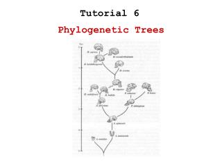
4. Primate evolution A phylogeny is a tree that describes the sequence of speciation events that lead to the forming of a set of current day species; also called a phylogenetic tree.

5. Theory of Evolution • Basic idea • speciation events lead to creation of different species. • Speciation caused by physical separation into groups where different genetic variants become dominant • Any two species share a (possibly distant) common ancestor

6. Aardvark Bison Chimp Dog Elephant Phylogenenetic trees • Leaves - current day species (or taxa – plural of taxon) • Internal vertices - hypothetical common ancestors • Edges length - “time” from one speciation to the next

7. Types of Trees A natural model to consider is that of rooted trees Common Ancestor

8. Types of trees Unrooted tree represents the same phylogeny without the root node Usually, data from current day species does not distinguish between different placements of the root.

9. Tree a Tree b Rooted versus unrooted trees Tree c b a c Represents the three rooted trees

10. Positioning Roots in Unrooted Trees • We can estimate the position of the root by introducing an outgroup: • a set of species that are definitely distant from all the species of interest Proposed root Falcon Aardvark Bison Chimp Dog Elephant

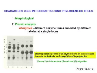
11. Morphological vs. Molecular • Classical phylogenetic analysis: morphological features: number of legs, lengths of legs, etc. • Modern biological methods allow to use molecular features • Gene sequences • Protein sequences • Analysis based on homologous sequences (e.g., globins) in different species

12. From sequences to a phylogenetic tree Rat QEPGGLVVPPTDA Rabbit QEPGGMVVPPTDA Gorilla QEPGGLVVPPTDA Cat REPGGLVVPPTEG There are many possible types of sequences to use (e.g. Mitochondrial vs Nuclear proteins).

13. Type of Data • Distance-based (The project focus on this method). • Input is a matrix of distances between species • Can be fraction of residue they disagree on, or alignment score between them, or … • Character-based • Examine each character (e.g., residue) separately Not covered in this project

14. Constructing trees from distances: • Transform differences between species to numerical distances • Find a weighted tree that realizes/approximates the distances between the species. The task is: Given a set of species (leaves in a supposed tree), and distances between them – construct a phylogeny which best “fits” the distances.

15. Exact solution: Additive sets Given a set S of n objects with an n×ndistance matrix: • d(i,i)=0, and for i≠j, d(i,j)>0 • d(i,j)=d(j,i). • For all i,j,k it holds that d(i,k) ≤ d(i,j)+d(j,k). Can we construct a weighted tree which realizes these distances?

16. k c b j v a i There is always a tree for 3 objects For n=3: There is always a (unique) tree with one internal node. Distance metrics on 4 objects may not have a tree.

17. k i l j The Four Points Condition Definition: A distance metric on n objectssatisfies the four points condition iff any subset of four objects can be labeled i,j,k,l so that: d(i,k) + d(j,l) = d(i,l) +d(k,j) ≥ d(i,j) + d(k,l) Theorem: A distance metric is additive , it satisfies the four points condition Note: The four point condition implies O(n4) algorithm, which is not very efficient.

18. Constructing additive trees:The neighbor joining problem Let i, j be neighboring leaves in a tree, let v be their parent, and let k be any other vertex. The formula shows that we can compute the distances of v to all other leaves. k d(k,v) v j i

19. Constructing additive trees:The neighbor joining problem • This suggest the following method to construct tree from a distance matrix: • Find neighboring leaves i,j in the tree, • Replace i,j by their parent v and recursively construct a tree T for the smaller set. • Add i,j as children of v in T.

20. A B C D Neighbor Finding How can we find from distances alone a pair of neighboring leaves (called also cherries)? Closest vertices aren’t necessarily neighboring leaves.

21. Neighbor Finding: Seitou&Nei method Definitions Theorem (Saitou&Nei)Assume all internal edge weights are positive. If Q(i,j) is minimal (among all pairs of leaves), then i and j are neighboring leaves in the tree.

22. k v i j S&N Neighbor Joining Algorithm • If n =3, return tree of three vertices • Compute Q(i,j) for all i,j • Choose i,j such that Q(i,j) is minimal • Create new vertex v, and set d(k,v) • remove i,j, and add v to the set of objects • Recursively construct a tree on the smaller set, then add i,j as children of v, at distances d(i,v) and d(j,v).

23. Complexity of S&N Neighbor Joining Algorithm Initialization:θ(n2) to compute r(i) and Q(i,j) for all i,jL. Each Iteration: • O(n2) to find the maximal Q(i,j). • O(n) to compute {D(v,k):k L} for the new node v, and to update the matrix. • O(n2) to update the values Q(i,j). Total of O(n3). k D(v,k) i j

24. Some remarks on S&N Neighbor Joining Algorithm • Applicable to matrices which are not additive • Known to work good in practice. • The algorithm and its variants are the most widely used distance-based algorithms today. Next we present a more efficient Neighbor Joining algorithm, which is based on LCA distances.

25. Least Common Ancestor distances Definition:Given a weighted tree T and a specific vertex r in it: dT(r;i j)=distance in T from r to path(i,j). dT(r;i i)=distance in T from r to i. r 3 5 Edge weights: 3 DT(r;AD)= 3 2 5 LCA distances: 2 5 D 3 2 2 1 5 E DT(r;AA)= 7 B A C 6 7 8 7

26. Least Common Ancestor distances The distances dT(r;i,j) can be presented by a matrix: r 3 5 5 5 D 6 7 7 E B A 8 C

27. LCA Matrices Definition: A symmetric nonnegative matrix L is an LCA matrix iff • For each i: L(i,i)=maxj{L(i,j)} • It satisfies the “3 points condition”: for each 3 distinct indices i, j, k , L(i,j) ≥ min {L(i,k), L(j,k)} “the smallest value appears twice”

28. LCA Matrices Theorem: The following conditions are equivalent for an (n-1)(n-1) matrix L: • L is an LCA matrix. • There is a weighted tree T with n leaves and a leaf r in T such that for each pair of leaves i,j  r: L(i,j)= dT(r;ij)

29. LCA distances LCA matrix There is a weighted tree T s.t. L(i,j)= dT(r;ij).  L is an LCA matrix: By properties of least common ancestors in trees r L(k,i) = L(j,i) L(k,j) j i k

30. LCA matrix LCA distances Now we are given an LCA matrix L and need to construct a tree.The construction uses “maximal off diagonal” entries: L(i,j) is a “maximal off-diagonal” in entry in row i if L(i,j)=maxk{L(i,k):k i} Example: L(1,2) is maximal off diagonal entry in row 1

31. Maximal off diagonal entries Lemma: If L(i,j) is the maximal “off-diagonal” entry in both rows i and j in L, then for all k i,j: L(i,k)=L(j,k). Proof: By the 3 points condition on {i,j,k}. Examplefor i=1, j=2

32. LCA matrix LCA distances:Proof by induction We now prove by induction on n: L is an (n-1)(n-1) LCA matrix There is a weighted tree T with a root r as in the theorem. Basis: n= 2. L=[w]. T is a tree with a single edge of weight w. 4 4 r i

33. Induction step Induction step: n ¸ 3. Let L be an LCA matrix of dimension n-1. We describe an algorithm for constructing the corresponding tree: 1. Find i,j s.t. L(i,j) is the maximal off-diagonal entry in L. L (In the example i=1andj=2)

34. Induction step 2. Let L` be the matrix obtained by removing rows/columns i and j, and inserting row/column v s.t. L`(v,v)=L(i,j), and for ki,j, L`(v,k)=L(i,k) (=L(j,k)) L` L

35. Induction Step To show that L` We is an LCA matrix we need a definition and a simple observation: Definition: Let L be an nn matrix, and let S  {1,...,n}. L[S] is the submatrix of L consisting of the rows and columns with indices from S. Observation 1: If L is an LCA matrix then for every S  {1,...,n}, L[S] is also an LCA matrix.

36. Induction step Claim: L` is an LCA matrix of dimension n-2 Proof: Let S be all leaves except j. Than L` is obtained from L(S) as follows: • change the index i to v • set L`(v,v)ÃL(i,j) By Observation 1 and the maximality of L(i,j), L` is also an LCA matrix. L` L

37. v Induction step 3. Construct a tree T` for L` (with n-1 leaves) L` T`

38. v Induction step 4. Add to v to childs, for i and j, with appropriate edge lengths. T` 2 5 i j

39. Deepest LCA neighbor joining • If n ·3, return tree of n vertices • Prepare a list MAX of size n, s.t. MAX(i ) = maximal off diagonal element in row i Recursion: • Find i,j s.t. L(i,j) is maximal off diagonal entry of L • Make the reduction to L` as described • update the list MAX (only MAX(v) needs an update!) • Construct T` for L` • Add i and j as childs of v. T` v i j

40. Complexity Analysis Initialization: Constructing MAX - O(n2). Let Time(n) be the complexity of the algorithm, given the input matrix L and the list MAX. Time(n) is given by: • Reducing L to L`: O(n) • Updating MAX: O(n). • Constructing T` from L`: T(n-1). • Constructing T from T`: O(1). Time(n)·Time(n-1)+O(n) Hence Time(n)=O(n2)

41. Seitou&Nei vs. DLCA methods • DLCA like S&N can be implemented on noisy data (in many ways) • On exact data, DLCA and S&N methods have the same (correct) output. They differ on noisy data (which occurs in practice). • One basic difference: Unlike S&N method, the DLCA algorithm depends on selecting a root. Hence DLCA may produce many different trees on the same output. Some of the projects will concentrate on this difference.

42. Incremental Reconstruction via Local Queries Incrementally reconstructing the tree: g f g f c e b 5 c e b 4 5 2 3 3 4 1 1 6 a 6 a 2 d d h h • When inserting a new taxon x to a given topology T, we need to find out to which edge x should be attached. • We are allowed to ask the ‘oracle’ local queries LQ(x,v). (x – taxon, v – internal vertex)

43. g f c e b 5 c e b 2 3 3 4 1 1 a 6 a 2 d d h Local Queries - Motivation • Asking LQ(x,v) is equivalent to asking the topology of {x, a, b, c}, where v is the center-point of a,b,c in T. f 4 • Such questions can be asked directly (using likelihood) or through a pairwise distance matrix (which will be discussed later)

44. Balancing Vertices • We’d like to minimize the number of queries required for inserting a new taxon. • Lower bound – log3(|ET|). (simple adversarial argument) • Upper bound – log2(|ET|). • The algorithm which achieves the upper bound uses ‘balancing vertices’: • A balancing vertex in T is an internal vertex, which splits T into 3 subtrees of size at most ceil(|T|/2). • Using balancing vertices in the local queries, the edge to which a new taxon should be attached can be found in ~ log2(|ET|) queries.

45. g f c e a d h Balancing Vertices • Every tree contains either a single balancing vertex or two adjacent balancing vertices. • Finding a balancing vertex: • Start at some arbitrary vertex v. • If v is balancing, stop. • Otherwise, continue to the vertex u, adjacent to v in the ‘heaviest’ subtree. • The algorithm traverses each edge at most once  Time complexity – O(|T|). 13 edges in T 11 edges 9 edges 7 edges

46. A Simple and Efficient Algorithm • Iteratively add taxa 1,2,…,n to the topology • When adding taxon x to topology T: • If T is trivial (consists of a single edge), attach x to that edge. • Otherwise: • Find a balancing vertex v of T. • Ask query LQ(v,x) • Continue recursively on T’, the subtree corresponding to the answer of the query. • Complexity: • Adding taxon 1≤x≤n to T takes O(log(x)) queries and O(x) time. • Total query complexity: O(n·log(n)) • Total time complexity: O(n2)

47. Interesting Issues • Two major issues are raised in this area: • Queries do not always have reliable answers • Use confidence level for answers • Verify the answers • Reduce running time to O(n·log(n)) • Finding balancing vertices leads to high overhead • Maybe we don’t have to re-compute the balancing vertices in every stage

48. Robustness to Noise in Data Answering local queries using a distance matrix D: • We wish to assess the topology spanned by four taxa: x, a, b, c. • Observe the 4×4 submatrix of D over x, a, b, c: b x a c c b b x ? a x a c • If D is additive then there is a labeling of the taxa by i, j, k, l s.t:D(i,j) + D(k,l) ≤ D(i,k) + D(j,l) = D(i,l) + D(j,k) • The configuration of the quartet is (ij ; kl), and the path separating them is of length ½(D(i,k) + D(j,l) - D(i,j) + D(k,l)) • If D is not additive we set the configuration of the quartet to (ij ; kl), where D(i,j) + D(k,l) is minimal of the three sums. • Confidence of prediction can be estimated by the difference between maximal and minimal sums.

49. Robustness to Noise in Data Answering local queries using a distance matrix D: • We can check several quartets of type x, a, b, c to answer a single local query.Example: To answer LQ(1,g) we can check all quartets in{g} ×{a} ×{c,f} ×{b,d,e} f c e b 4 2 3 ? 1 g a d • We can choose a representative set of quartets, and answer the local query according to (weighted) majority. • If the answer is still inconclusive, we can choose to ask another local query.

50. 4 T: S: l m 6 6 j 3 e k f 5 2 d 3 g i c 2 1 5 1 4 a h b a b c d e f g h i j k l m Improving Running Time Separator Trees: • A deterministic algorithm which inserts a new taxon x to a given topology T can be viewed as a rooted decision tree. • Each internal node represents a local query (internal vertex in T). • Each internal node has three outgoing edges corresponding to the three possible answers to the query. • Each leaf corresponds to an edge in T. • A special case of decision trees are separator trees. The time complexity of the algorithm is the depth of the separator tree